A Look at Typed Lambda Calculus

This is the second article in our short series on lambda calculus. If you are unfamiliar with lambda calculus, we recommend starting with the first article. In this piece, we focus on introducing types to lambda calculus.

We’ve also previously covered the history of formal verification and, by extension, type theory. Reading that article might provide a historical background for the topics we’ll discuss here.

We assume familiarity with the basic lambda calculus syntax, which we covered in the previous article. Additionally, we assume basic understanding of the related concepts, including unrestricted computation, logic systems, paradoxes, Russell’s type theory, and logical consistency.

Typed lambda calculus extends the untyped lambda calculus by introducing a type system. It’s important to note that, unlike untyped lambda calculus, there are multiple typed lambda calculi, each differentiated by the specific features of the type system used. The exact features of the type system can be chosen with considerable flexibility. In this article, we will explore some of the common choices.

The untyped lambda calculus is hard to use as a logic system due to the paradoxes it creates. Adding Russell’s type theory to lambda calculus makes it, under certain conditions, logically consistent, which, in turn, makes it possible to mathematically guarantee certain behaviors (or lack thereof).

The most common argument for the strongly-typed languages is that if a program type checks, it will never segfault (or have any other type-related issues), but I think this argument sells typed languages short. A sufficiently strict and expressive type system allows for encoding much more than simply “not segfaulting.” In some cases, the whole domain can be expressed in types.

In this article, we are primarily focused on the basics, and therefore, we won’t delve deeply into the more expressive type systems such as System FC or those with dependent types.

Simply typed lambda calculus with atomic boolean values

Well-Typed Expressions Do Not Go Wrong

– Robin Milner, “A Theory of Type Polymorphism in Programming”

We will now introduce atomic values to the lambda calculus. While it is feasible to construct a value representation using only λ-abstractions (using Church encoding or otherwise) for almost any value we might be interested in, practically speaking, it’s not very convenient, rather memory-inefficient, and performance of the Church encoding on modern systems isn’t great.

Thus, we introduce atomic values $true$ and $false$.

Since we’ve introduced atomic values, we also need to introduce an eliminator (i.e. a consumer) for these values. In this case, let’s consider an $\mathbf{if} \ldots \mathbf{then} \ldots \mathbf{else} \ldots$ operator.

The semantics of this operator should be reasonably familiar to a practicing programmer, but let’s informally write them them out anyway:

• $\mathbf{if}\; true\; \mathbf{then}\;\alpha\;\mathbf{else} \;\beta$ should reduce to $\alpha,$
• $\mathbf{if}\; false\; \mathbf{then}\;\alpha\;\mathbf{else} \;\beta$ should reduce to $\beta,$
• $\mathbf{if}\; \gamma\; \mathbf{then}\;\alpha\;\mathbf{else} \;\beta$ where $\gamma$ is a redex, $\gamma$ should be reduced first.

The introduction of the $\mathbf{if}$ operator creates a bit of a kink. What do we do if $\gamma$ is neither $true$, $false$, nor a redex? E.g. $\mathbf{if}\; (\lambda x. x)\; \mathbf{then}\;\ldots\;\mathbf{else} \;\ldots$

Such terms are called “stuck” — the computation, according to our rules, can not proceed.

We want to avoid stuck terms!

To do that, we’ll have to place some restrictions on what $\gamma$ could be.

Typing relations, rules, and systems

To express such restrictions, we introduce the so-called typing relation. A typing relation is a relation, in this case meaning a set of pairs, which assigns types to syntactically valid terms.

Not all syntactically valid terms can have a type assigned to them. We call terms that have a type well-typed, and the others ill-typed. The point of having a type system is to reject ill-typed terms, as those are the ones likely to get “stuck”.

One such individual assignment we’ll call a typing judgement, and will write it separated by a column: $t : T$, read as “term $t$ has type $T$”.

Types can be thought of as sets of terms of a certain general form. Turns out (Reynolds, 1984), this naive interpretation of types as sets doesn’t hold to rigorous scrutiny. Still, it’s a good enough mental model unless you’re a type theory researcher (and if you are, hi, very nice of you to read this article, please get in touch if you have corrections).

In most practically relevant cases, specifying the typing relation by direct enumeration is at best impractical, and is usually impossible. We can instead specify it by writing out a finite set of rules, called typing rules, from which the typing relation can be derived. Together, types and typing rules constitute a type system.

Type systems offer a lightweight (i.e. without executing a program) tool to check if a program is “correct” – in a sense that it doesn’t produce stuck terms.

Typing rules are usually written in the form

$$\begin{array}{c} \text{premises} \\ \hline \text{conclusion} \end{array}$$

where $\text{premises}$ is zero or more semicolon-separated typing judgements, and $\text{conclusion}$ is a single typing judgement.

If there are no premises, i.e. the conclusion is an axiom, the horizontal line is often omitted.

Let us introduce the type $Bool,$ which represents a set of $true,$ $false,$ and any redexes that eventually evaluate to either.

Now we can write typing rules for our boolean values $true$ and $false$ as axioms:

$$\begin{array}{lll} true : Bool & \text{(AxT)} \\ false : Bool & \text{(AxF)} \end{array}$$

And for the $\mathbf{if}$ operator:

$$\begin{array}{cc} \begin{array}{c} t_1 : Bool;\quad t_2 : T;\quad t_3 : T \\ \hline \mathbf{if}\;t_1\;\mathbf{then}\;t_2\;\mathbf{else}\;t_3 : T \end{array} & \text{(If)} \end{array}$$

Note that rules are annotated with names. We’ll use these names to reference the rules later.

The first two rules, $\text{(AxT)}$ and $\text{(AxF)},$ are trivial. The third rule, $\text{(If)}$, reads “given that $t_1$ has type $Bool$, and both $t_2$ and $t_3$ have the same arbitrary type $T$, then $\mathbf{if}\;t_1\;\mathbf{then}\;t_2\;\mathbf{else}\;t_3$ has this type $T$”.

We should note that the $\text{(If)}$ typing rule will forbid some “correct” terms, as in “terms that aren’t stuck”. For example, $\mathbf{if}\;true\;\mathbf{then}\;true\;\mathbf{else}\;(\lambda x.\; x)$ is just $true$, which is arguably perfectly reasonable, but our type system wouldn’t allow it.

This is true in general: any sufficiently strict type system will reject some “correct” terms, but that’s basically a consequence of Gödel’s incompleteness theorems, so either we have to deal with a system that allows for paradoxes (inconsistency), or we have to live with some arguably correct terms being rejected (incompleteness).

In this particular example, it makes sense if you think about it. The example above is trivial enough, but consider you might have $\mathbf{if}\;\text{<long and hard computation>}\;\mathbf{then}\;true\;\mathbf{else}\;(\lambda x.\; x).$ Here, it is quite unclear what the type of the whole expression should be without executing the program. That is not to say this is a fundamental restriction, more powerful type systems can lift it, but we won’t discuss them here.

We call a type system sound if it assigns (relates) at most one type to each term.

Typing lambda-abstractions, variables and applications

We have introduced typing rules for boolean values and $\mathbf{if}$, but there are other terms in our calculus. Specifically, we also have abstractions, applications, and variables.

Let’s start with abstractions.

A lambda-abstraction is basically a function of a single argument. We could introduce a new simple type $Abs$ and relate all abstractions to this type. Unfortunately, we would soon run into trouble with this approach.

Indeed, imagine a term $\mathbf{if}\;true\;\mathbf{then}\;(λx.\;true)\;\mathbf{else}\;(λx.\;λy.\;y).$ Both branches would have the type $Abs$, but their behavior is very different. This example suggests that we need to know both the argument type and the return type of a lambda abstraction.

So instead of a single type, we introduce a family of types $T_1 \to T_2,$ where $\to$ is a type constructor. A type $T \to U$ relates to all functions accepting an argument of type $T$ and returning the result of type $U.$ For the sake of simplicity of notation, we assume $\to$ is right-associative, hence to write the type of an abstraction returning an abstraction, e.g. $T \to (U\to V),$ we don’t need parentheses, i.e. $T \to U \to V$.

To decide on the argument type, we basically have two options:

• We can try to “guess” what type it should be based on context. This is inferred typing. Not always possible, though.
• We can demand that the type is specified explicitly. This is explicit typing.

For now, let’s go with the second option. Hence, we need to introduce an explicit typing notation:

$$\lambda x : T. \; \ldots$$

All λ-abstractions must be explicitly typed like this.

If we know the type of the abstraction argument, we can infer the type of the result by substituting the known type of the variable into the typing rules for the abstraction body. Formally, this idea is expressed by introducing a typing context.

A typing context is a set of typing judgements for variables that are “in scope”, i.e. judgements that are locally known but not necessarily globally true. Note that variables are not assumed to be identified by their names here: each variable will have a corresponding distinct typing judgement in the context even if their names are the same.

Practically speaking, typing context can be thought of as a mapping from variables to types and is often implemented as such.

The “current” context is usually denoted by $\Gamma,$ and is written to the left of other typing judgements, separated by $\vdash$ (a symbol for logical entailment). We can also extend the context by simply adding new comma-separated typing judgements, e.g. $\Gamma, x : T$ is the context $\Gamma$, extended by the judgement $x:T.$

Using all this new syntax, we can define a typing rule for abstractions now:

$$\begin{array}{c} \Gamma, x:T_1 \vdash t : T_2 \\ \hline \Gamma \vdash \lambda x:T_1.\; t : T_1 \to T_2 \end{array}\quad\text{(Abs)}$$

This rule simply says that if – given the current context plus the type of the abstraction variable $T_1$ – the type of the body turns out to be $T_2$, then the whole abstraction in the current context has type $T_1 \to T_2.$ Pretty straightforward, but the notation may seem a bit arcane. Spend a minute to understand it, we’ll be using it more down the line.

For individual variables, the typing rule would then be rather trivial:

$$\begin{array}{c} x : T \in \Gamma \\ \hline \Gamma \vdash x : T \end{array}\quad\text{(Var)}$$

For applications, it’s a bit more involved, but hopefully nothing too surprising:

$$\begin{array}{c} \Gamma \vdash t_1 : T_1 \to T_2;\quad \Gamma\vdash t_2 : T_1 \\ \hline \Gamma \vdash t_1\; t_2 : T_2 \end{array}\quad\text{(App)}$$

Try to interpret this one yourself, then check if you’re correct.

Answer

This reads, basically, "for an application expression, if the left-hand side (function) has type $T_1\to T_2,$ and the right-hand-side (argument) has the type $T_1$, then the result of the application will have type $T_2.$

---

To clear up a technicality, we also need to have the context in our $\text{(If)}$ rule, since typings of terms might depend on the context, too:

$$\begin{array}{cc} \begin{array}{c} \Gamma\vdash t_1 : Bool;\quad \Gamma\vdash t_2 : T;\quad \Gamma\vdash t_3 : T \\ \hline \Gamma\vdash\mathbf{if}\;t_1\;\mathbf{then}\;t_2\;\mathbf{else}\;t_3 : T \end{array} & \text{(If)} \end{array}$$

Example

The practical application of these rules is we can use those to assign types to terms and thus ensure the program doesn’t get stuck.

In actual practice, we’d have some inference algorithm to decide on types of terms (and whether they have one). In this theoretical introduction, we’ll just assume there’s some way to get the type of a given term, without getting into the specifics of how it works.

As a proof that a given term has a given type, we can use typing trees. Typing trees just chain typing rules in a tree-like structure.

As a simple example, let us show that term $(\lambda x: Bool.\; x)\;true$ has type $Bool$ in some arbitrary context $\Gamma$.

$$\begin{array}{c} \begin{array}{c} \begin{array}{c} x : Bool \in \Gamma, x:Bool \\\hline \Gamma, x:Bool \vdash x : Bool \end{array}\quad\text{(Var)} \\\hline \Gamma \vdash (\lambda x:Bool.\; x) : Bool \to Bool; \end{array}\begin{array}{c}\\\text{(Abs)}\end{array} \quad \begin{array}{c} \\\\\Gamma \vdash true : Bool \quad\text{(AxT)} \end{array}\\ \hline \Gamma \vdash (\lambda x:Bool.\; x)\; true : Bool \end{array}\quad\begin{array}{c}\\\\\text{(App)}\end{array}$$

It may be more natural to read this typing tree bottom-up. We start with the initial premise, i.e. the expression in question has the expected type. This is justified by the $\text{App}$ rule, where $t_1$ is instantiated (i.e. replaced) with $(\lambda x:Bool.\; x)$, $t_2$ with $true$, $T_1$ and $T_2$ with $Bool$. The second premise of the $\text{App}$ rule, namely that $true: Bool$, is trivially true due to $\text{AxT}$. The first premise is true due to the $\text{Abs}$ rule, wherein $T_1$ and $T_2$ are instantiated with $Bool$, and $t$ with $x$. The premise of the $\text{Abs}$ rule in turn is true due to the $\text{Var}$ rule, as the judgement $x:Bool$ is trivially an element of the typing context $\Gamma, x: Bool$ (i.e. an arbitrary context $\Gamma$ extended by the judgement $x: Bool$).

Actual inference algorithms ultimately constructively build such proofs. However, there isn’t necessarily a single way to build them: a given type system may have multiple inference algorithms. On the other hand, a type system may be sound, but undecidable, in which case it will not have a general inference algorithm at all.

The impossibility of simply typed lambda calculus without atomic values

So, we have a sound type system. However, it does have one pretty obvious drawback.

On the soundness

We will omit the proof of the soundness of the simply typed lambda calculus with atomic booleans, however, it’s easy enough to find for the interested reader, e.g. in (Pierce, 2002).

The short sketch is to prove soundness we need to prove two propositions:

1. A typed term can not be stuck.
2. If a typed term is beta-reduced, the result is also a typed term.

Both are proven by structural induction on terms, but you’ll also have to formally define the computation semantics, which here we glossed over.

---

In the untyped lambda calculus, we could define

$$id = \lambda x.\; x$$

and use it anywhere we would fancy an identity function.

With our new fancy type system, we can not. Obviously, for any concrete type, we could define

$$id_{Bool} = \lambda x : Bool.\; x,$$

$$id_{Bool \to Bool} = \lambda x : Bool \to Bool.\; x,$$

$$\ldots$$

But we can’t do it in general.

Notice how we need a terminating type in the type signature. Consequently, if our calculus didn’t have any atomic values, i.e. didn’t have any types beyond abstractions, we wouldn’t be able to specify the argument type.

The reason for this is the lack of polymorphism.

Polymorphic lambda-calculi

Double-barreled names in science may be special for two reasons: some belong to ideas so subtle that they required two collaborators to develop; and some belong to ideas so sublime that they possess two independent discoverers. […] the Hindley-Milner type system and the Girard-Reynolds polymorphic lambda calculus [are the] ideas of the second sort.

– Philip Wadler, “The Girard-Reynolds Isomorphism”

Polymorphism, essentially, is the ability of the type system to deal with terms that can have arbitrary types. Practically speaking, a fully-typed program will not have any terms with polymorphic types, as a polymorphic type is basically a placeholder to be replaced with concrete types during compilation.

But parts of a program, especially during type checking or type inference, might have polymorphic types.

On polymorphic types as placeholders

Viewing polymorphic types as placeholders to be replaced is justified in the context of this theoretical introduction, and it gives a useful intuition. However, in practice, things like dynamic dispatch make it a bit more complicated.

---

We need to distinguish two different kinds of polymorphism (Strachey, 2000):

• Ad-hoc, which defines a common interface for an arbitrary set of individually specified types, and
• Parametric, which allows using abstract symbols in type signatures, representing arbitrary types, instead of concrete types.

Ad-hoc polymorphism is more common, and is used extensively in popular programming languages like C++, Java, etc, where it’s called “function/method/operator overloading.” Essentially, ad-hoc polymorphism is a way to make a single function (or, more accurately, a single API endpoint) behave differently for different types. For example, summing integers is pretty different from floating-point numbers, but using a single operator for both is convenient.

Parametric polymorphism is a bit different: it allows us to use so-called type variables in the type signature. At the use site, type variables are instantiated to concrete types. The implementation must be the same regardless of the specific instantiation.

Ad-hoc polymorphism is, generally speaking, pretty ad-hoc. It doesn’t have much of a theoretical background to speak of, although there’s an approach to making it less ad-hoc (Wadler, 1989). In contrast, parametric polymorphism does have a strong theoretical foundation.

Hindley-Milner type system

First, let us discuss the so-called rank-1 polymorphism.

We introduce type variables using the universal quantifier, $\forall.$ The exact place where the variables are introduced matters.

In particular, rank-1 polymorphism allows the universal quantifier only on the top level of types. Practically, this means that $\forall \alpha.\;\alpha \to \alpha$ is okay, but $\forall \beta.\;(\forall \alpha.\;\alpha \to \alpha)\to \beta \to \beta$ is not.

There’s an argument to be made about how $Bool\to (\forall \alpha.\; \alpha \to Bool)$ is practically rank-1 polymorphic as it is isomorphic to $\forall \alpha.\;Bool\to \alpha \to Bool,$ but we’ll gloss over this point here.

Rank-1 polymorphic type system with type inference is first described by Roger Hindley in (Hindley, 1969), and later rediscovered by Robin Milner in (Milner, 1978).

A formal analysis and correctness proof was later performed by Luis Damas in (Damas, 1982).

This type system is called the Damas-Hindley-Milner type system, or more commonly the Hindley-Milner type system. We will call it HM below.

HM (usually with many extensions) is used as a base for many functional languages, including ML (by the way invented by Robin Milner) and Haskell.

On Haskell's type system

I say HM is used as a base for Haskell. This is on some technical level correct, but I feel a deluge of “um, actually” coming, so I’ll get this out of the way. For a while, Haskell used a variation of System Fω at the back end, at some point switching to System FC, while on the front end both Haskell98 and Haskell2010 use a variation on HM with type classes and monomorphism restriction. If we include various GHC extensions, things quickly get very complicated, but at the core, it’s still somewhat similar to HM.

---

Let-polymorphism

HM makes one concession for the sake of type inference. It only allows the so-called let-polymorphism instead of unconstrained parametric polymorphism.

To explain what this means with an example: one would like to have polymorphic type inference for expressions like

$$(\lambda id.\; \ldots (id\;true) \ldots (id\;123) \ldots)\;(\lambda x.\; x),$$

but type inference in polymorphic lambda calculus is in general undecidable without explicit type annotations (Wells, 1999).

To work around that, HM stipulates that polymorphic types can only be inferred for let-bindings, e.g. bindings of the form

$$\begin{array}{rl} \mathbf{let} & id = \lambda x.\; x\\ \mathbf{in} & \ldots (id\;true) \ldots (id\;123) \ldots \end{array}$$

Obviously, HM has to introduce the let-binding construction into lambda calculus syntax and define its semantics in terms of base lambda calculus. Hopefully, the translation is more or less obvious – let-bindings are semantically equivalent to immediately-applied lambda abstractions. Note, however, that this doesn’t yet allow for recursive definitions.

HM syntax

I will now formally introduce the syntax of expressions, types, and a function $free$ acting on type expressions. I’ll use an informal variation of BNF (Backus-Naur form) to define syntax.

The expression syntax is exactly the syntax of lambda calculus plus the let-in construct:

$$\begin{array}{rrll} t & ::= & x & \text{variable} \\ & | & t_1\;t_2 & \text{application} \\ & | & \lambda x.\; t & \text{abstraction} \\ & | & \mathbf{let}\; x = t_1\;\mathbf{in}\;t_2 & \text{let-in} \end{array}$$

Note that $t$, $t_1$, $t_2$ are recursive references.

Types are introduced in two parts, the first part being the monotypes $\tau$ and the second – polytypes $\sigma$ (also called type schemes, hence the $\sigma$):

$$\begin{array}{rrll} \tau & ::= & \alpha & \text{type variable} \\ & | & C\;\tau_1\;\ldots\;\tau_n & \text{type constructor application} \\\sigma & ::= & \tau & \text{monotype} \\ & | & \forall \alpha .\; \sigma & \text{quantified type} \end{array}$$

$C$ represents type constructors, defined as primitives, and their set is arbitrary in HM, but it must include at least the abstraction type constructor $\to$.

Parentheses can be used in value and type expressions to change evaluation order, but we omit these in the syntax definitions for brevity.

Note that type variables are admitted as monotypes, which makes those distinct from monomorphic types that can’t have type variables.

Polytypes also include monotypes, in addition to quantified types.

The quantifier $\forall$ binds the type variables, so in a type expression $\forall \alpha_1\;\ldots\;\alpha_n.\; \tau,$ all of $\alpha_i$ are bound. Type variables that are not bound are called free.

The crucial difference between monotypes and polytypes is the notion of equivalence.

Monotypes are considered equivalent if they are syntactically the same, i.e. have the same terms in the same places. So, for example, a monotype $\alpha$ is only equivalent to $\alpha,$ i.e. itself.

With polytypes, the equivalence is considered up to the renaming of bound variables (assuming no conflicts with free type variables of course). So, for example, $\forall \alpha. \alpha \to \beta$ is equivalent to $\forall \gamma. \gamma \to \beta.$

Notice we couldn’t rename $\alpha$ to $\beta$, as that would result in an entirely different polytype – this is the same quirk as with α-equivalence of abstractions in untyped λ-calculus.

We also need a function $free$ to define typing rules. $free$ collects all free variables from its argument. It is defined as follows:

$$\begin{array}{lcl} free(\alpha) & = & \{\alpha\} \\ free(C\;\tau_1\;\ldots\;\tau_n) & = & \bigcup\limits_{i=1}^n free(\tau_i) \\ free(\forall \alpha.\; \sigma) & = & free(\sigma) - \{\alpha\} \\ free(\Gamma) & = & \bigcup\limits_{x:\sigma \in \Gamma} free(\sigma) \\ \end{array}$$

The function is properly defined on type expressions (i.e. polytypes and consequently monotypes). However, for notational convenience the last equation extends it also to typing contexts.

The principal type

Polymorphism implies that the same term can have more than one type. In fact, it could have infinitely many types, as is the case with $\lambda x.\; x.$

For the type system to be sound, we need to somehow choose the “most best” type out of all possibilities. Thankfully, there is a straightforward way to do so.

The idea is to choose the largest most general type, also called the principal type – that is, the most specific polytype that can still produce any other possible type via bound variable substitution. We denote substitution of a type variable $\alpha$ for a monotype $\tau$ in an expression $e$ as $\{\alpha \mapsto \tau\}e.$

If some type $\tau'$ can be produced from $\tau$ by substitution, it is said that $\tau$ is more general than $\tau',$ written as $\tau \sqsubseteq \tau'.$ $\sqsubseteq$ defines a partial order on types.

Note that the more general type is “smaller” than the less general type. This is a feature of treating types as sets: the more general the type, the fewer possible values it can have. The most general type $\forall\alpha.\;\alpha$ is usually considered uninhabited (with a few caveats), i.e. it has no values at all.

Formally, this all can be expressed by the following rule (called specialization rule):

$$\begin{array}{c} \beta_i \notin free(\forall\alpha_1\ldots\alpha_n.\;\tau) \\ \hline \forall\alpha_1\ldots\alpha_n.\;\tau \sqsubseteq \forall\beta_1\ldots\beta_m.\;\{\alpha_i\mapsto\tau_i\}\tau \end{array}$$

where $\tau_i \in \{\tau_1, \ldots, \tau_n\},$ and each of $\tau_i$ can mention type variables $\beta_j.$

This rule essentially says that a more general type can be made less general by substitution.

The $\beta_i \notin free(\forall\alpha_1\ldots\alpha_n.\;\tau)$ condition ensures that free variables are not accidentally replaced and are treated as constants.

Typing rules

The complete HM ruleset is as follows:

$$\begin{array}{cl} \begin{array}{c}x:\sigma\in\Gamma\\\hline \Gamma\vdash x:\sigma\end{array} & \text{variable} \\ \begin{array}{c}\Gamma\vdash t_0:\tau\to\tau';\quad\Gamma\vdash t_1:\tau\\\hline \Gamma\vdash t_0\;t_1:\tau'\end{array} & \text{application} \\ \begin{array}{c}\Gamma,\;x:\tau\vdash t:\tau'\\\hline \Gamma\vdash \lambda x.\; t:\tau\to\tau'\end{array} & \text{abstraction} \\ \begin{array}{c}\Gamma\vdash t_0:\sigma;\quad\Gamma,\;x:\sigma\vdash t_1:\tau\\\hline \Gamma\vdash \mathbf{let}\;x = t_0\;\mathbf{in}\; t_1 : \tau\end{array} & \text{let-in} \\ \begin{array}{c}\Gamma\vdash t:\sigma';\quad\sigma'\sqsubseteq\sigma\\\hline \Gamma\vdash t : \sigma\end{array} & \text{instantiation} \\ \begin{array}{c}\Gamma\vdash t:\sigma;\quad\alpha\notin free(\Gamma)\\\hline \Gamma\vdash t : \forall \alpha.\;\sigma\end{array} & \text{generalization} \\ \end{array}$$

This is just one possible formulation of the ruleset. Other equivalent formulations exist, but this one is enough for our purposes for now.

Variable, application, and abstraction rules should already look somewhat familiar – indeed, those are almost exactly the same as those in simply typed lambda calculus.

One notable feature is that the variable rule allows variables to have polytypes, while application and abstraction do not. This, together with the let-in rule, enforces the constraint that only let-in bindings are inferred as polymorphic.

The let-in rule is unsurprisingly similar to a combination of application and abstraction rules. In fact, if we do combine them as follows:

$$\begin{array}{c} \Gamma\vdash t_0:\tau;\quad\Gamma,\;x:\tau\vdash t_1:\tau'\\\hline \Gamma\vdash (\lambda x.\; t_1)\;t_0:\tau' \end{array}$$

we see that the only substantial difference is $\text{let-in}$ uses the polytype $\sigma$ instead of the monotype $\tau$ for the type of $x.$

The last two rules deserve a bit of a closer look.

The instantiation rule says that if a given expression $t$ has a general type $\sigma'$ in context, it can be specialized to a less general type $\sigma,$ as defined in the previous subsection. This rule ensures we can in fact use $id : \forall\alpha.\;\alpha\to\alpha$ in any matching context, e.g. $Bool\to Bool.$

On the other hand, the generalization rule works kind of in reverse: it adds a universal quantifier to a polytype. The idea here is that an implicit quantification in $\Gamma\vdash t:\sigma$ can be made explicit if the type variable in question $\alpha$ does not appear free in the context. The immediate consequence of this rule is that variables that end up free in a typing judgement are implicitly universally quantified.

Instantiation and generalization rules working together allow for essentially moving quantifications to the top level of a type.

Indeed, as polytypes are allowed neither in abstactions nor applications, when a polytype would occur there, instantiation rule would need to be used, replacing bound type variables with fresh free ones. Conversely, whenever a monotype with free variables occurs in a polytype position, generalization rule can be used to quantify them again.

Recursive bindings

In the discussion so far, we glossed over recursive bindings.

The original paper mentions recursion can be implemented using the fixed-point combinator $fix$.

Its semantics are pretty much the same as in untyped lambda calculus, and its type is

$$fix : \forall\alpha.\;(\alpha\to\alpha)\to\alpha$$

Note that this combinator can not be defined (or rather, typed) in terms of HM, so it has to be introduced as a built-in primitive.

Then, the syntactical form for recursive bindings can be introduced as syntactic sugar:

$$\mathbf{rec}\;v = t_1\;\mathbf{in}\;t_2 \equiv \mathbf{let}\;v = fix\;(\lambda v.\;t_1)\;\mathbf{in}\;t_2$$

Alternatively, an extension to the typing ruleset with the same semantics is possible.

This is all rather straightforward, but it comes at a price. With the introduction of $fix,$ non-terminating terms can be formulated, which otherwise isn’t the case.

For example, the term $fix\;id : \forall\alpha.\;\alpha,$ where $id$ is the identity function, is a non-terminating computation.

Additionally, as evidenced above, $\forall\alpha.\;\alpha$ becomes inhabited. This introduces various logical consistency issues, which are not usually an issue for a general-purpose programming language but are an issue for a theorem prover.

However, without $fix$, general recursion is not possible, which makes the calculus strictly less powerful than a Turing machine.

Hence, a choice has to be made either in favor of logical correctness or computational power.

System F

Hindley-Milner type system is nice in that it can infer types, but it is somewhat restrictive due to only supporting let-polymorphism.

One somewhat annoying feature is that, as discussed above, Hindley-Milner can not type the following term:

$$\lambda\;id.\; pair\; (id\; true)\; (id\; 4)$$

This comes down to type inference for higher-rank polymorphism being undecidable, but this issue is readily alleviated by explicit type signatures.

System F, independently discovered by Jean-Yves Girard (Girard, 1972) and John Reynolds (Reynolds, 1974), also called polymorphic lambda calculus or second-order lambda calculus, is a generalization of Hindley-Milner type system to arbitrary-rank polymorphism.

System F, unlike Hindley-Milner, formalizes parametric polymorphism explicitly in the calculus itself, introducing value-level lambda-abstractions over types. This essentially makes specialization explicit.

We will sketch the basics of System F here but won’t get into any detail. An interested reader is highly encouraged to look into (Pierce, 2002).

The primary new syntactical form introduced in F is the abstraction over types, denoted with a capital lambda: $\Lambda\alpha.\; t$

Since there is type abstraction, there is also type application, denoted as $t\;[\tau],$ where $t$ is a term and $\tau$ is a type. Square brackets are used to visually disambiguate type applications from term applications and don’t have any special meaning.

Syntax for types is similar to HM, but it’s not split into monotypes and polytypes, meaning universal quantification may appear anywhere in the type, not just on the top level:

$$\begin{array}{rrll} \tau & ::= & \alpha & \text{type variable} \\ & | & \tau_1\to\tau_2 & \text{function type} \\ & | & \forall \alpha .\; \tau & \text{quantified type} \end{array}$$

Typing rules are that of simply typed lambda calculus with the addition of

$$\begin{array}{cl} \begin{array}{c} \Gamma\vdash t:\forall\alpha.\;\tau_1\\ \hline \Gamma\vdash t\;[\tau_2]:\{\alpha\mapsto\tau_2\}\tau_1 \end{array} & \text{type application} \\ \begin{array}{c} \Gamma\vdash t:\tau;\quad\alpha\notin free(\Gamma)\\ \hline \Gamma\vdash \Lambda\alpha.\;t : \forall\alpha.\;\tau \end{array} & \text{type abstraction} \end{array}$$

(compare with instantiation and generalization rules in HM)

Hence, assuming $pair : \forall\alpha.\;\forall\beta.\;\alpha\to\beta\to Pair\;\alpha\;\beta,$ where the $Pair$ type constructor is assumed to be a primitive for simplicity, the motivating example could be typed as

$$(\forall\alpha.\; \alpha\to\alpha)\to Pair\;Bool\;Int,$$

and its actual implementation would use type applications explicitly, i.e.

$$\lambda\;id:\forall\alpha.\alpha\to\alpha.\; pair\;[Bool]\;[Int]\; (id\;[Bool]\;true)\; (id\;[Int]\;4)$$

On assuming Pair is a primitive

Polymorphic lambda calculi, unlike STLC, are powerful enough to admit Church encodings again. For instance, we could define the pair type as

$$Pair\;\alpha\;\beta = \forall \rho. (\alpha\to\beta\to\rho) \to \rho$$

and producers and eliminators for it as

$$\begin{align*} pair &= \Lambda \alpha. \Lambda \beta. \lambda x: \alpha. \lambda y: \beta. \Lambda \rho. \lambda s: \alpha \to \beta \to \rho. s\;x\;y\\ fst &= \Lambda \alpha. \Lambda \beta. \lambda p: Pair\;\alpha\;\beta. p\;[\alpha]\;(\lambda x:\alpha. \lambda y:\beta. x)\\ snd &= \Lambda \alpha. \Lambda \beta. \lambda p: Pair\;\alpha\;\beta. p\;[\beta]\;(\lambda x:\alpha. \lambda y:\beta. y) \end{align*}$$

with their types correspondingly

$$\begin{align*} pair &: \forall\alpha. \forall \beta. \alpha \to \beta \to Pair\;\alpha\;\beta\\ fst &: \forall \alpha. \forall \beta. Pair\;\alpha\;\beta \to \alpha\\ snd &: \forall \alpha. \forall \beta. Pair\;\alpha\;\beta \to \beta\\ \end{align*}$$

Of course, it’s still inefficient, so practical applications of this encoding are limited. Still, it’s nice that we can limit the base calculus to only have the $\to$ type constructor, and not lose anything in terms of expressive power.

In practical applications (like Haskell with RankNTypes extension), these explicit applications are inferred from type signatures. In GHC, they can also be made explicit with the TypeApplications extension.

The lambda cube

With System F, we’ve introduced the concept of terms depending on types via the type abstraction.

A natural question that might come from this is, what other kinds of dependencies might we introduce?

Dependence of terms on terms is a given since it’s a feature of untyped lambda calculus. But we can also have dependence of terms upon types, types upon terms, and types upon types.

Essentially, we have three axes, so this whole variant space constitutes, topologically speaking, a cube.

Behold, the lambda cube:

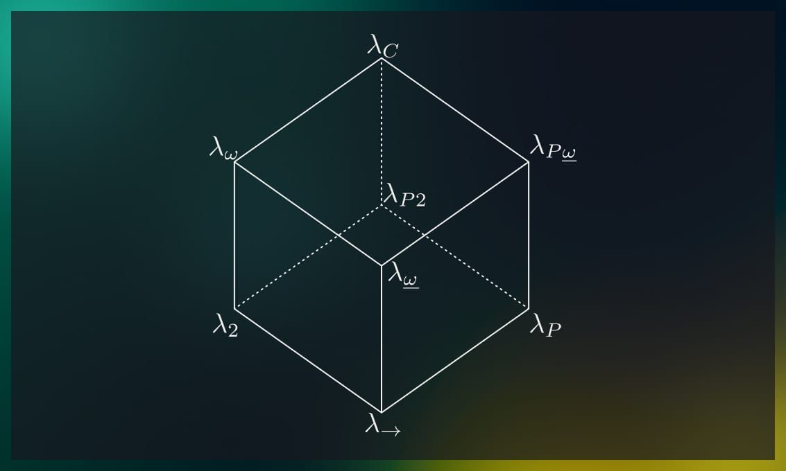
Going directly up in the picture introduces dependence of types upon types, i.e. user-defined type constructors.

Going left introduces dependence of terms upon types, i.e. System F style polymorphism.

Going right introduces dependence of types upon terms, i.e. Martin-Löf style dependent types.

Thus, we have the following variations:

	term ← type	type ← type	type ← term
$\lambda_\to$
$\lambda_2$	×
$\lambda_{\underline\omega}$		×
$\lambda_P$			×
$\lambda_\omega$	×	×
$\lambda_{P2}$	×		×
$\lambda_{P\underline\omega}$		×	×
$\lambda_C$	×	×	×

The left arrow ← denotes “depends on”.

The lambda cube was introduced by Henk Barendregt in (Barendregt, 1991) to investigate different generalizations of simply-typed lambda calculus (here denoted as $\lambda_\to$).

Let us briefly discuss some of the options.

$\lambda_2$ is System F, discussed above.

$\lambda_\omega$ is System Fω. It extends System F with type operators, which makes it much more complex, but also more expressive. In short, System Fω additionally allows quantification, abstraction and application for type constructors, essentially turning the type level into a simply-typed λ-calculus in its own right.

$\lambda_{\underline\omega}$, a.k.a. System Fω is System Fω without type abstraction/application on the term level. Practicall speaking, this boils down to simply typed lambda calculus with user-defined types.

$\lambda_P$ is simply typed lambda calculus with dependent types.

$\lambda_C$, a.k.a. $\lambda_{P\omega},$ is the calculus of constructions (Coquand, 1986), famously used as the base for the Coq proof assistant, but also with other dependently-typed languages. Here, the border between terms and types is virtually gone.

We will not discuss these advanced type systems in any more detail here, but I thought I should at least mention them.

Conclusions

We need to develop our insight into computing processes and to recognise and isolate the central concepts […]. To do this we must become familiar with them and give them names even before we are really satisfied that we have described them precisely.

– Christopher Strachey, “Fundamental Concepts in Programming Languages”

The topic of type theory is rather vast, so it’s infeasible to cover it in a single blog article in any considerable detail.

Hopefully, I’ve introduced enough basics here so that an interested reader can continue exploring this topic on their own, and mentioned enough topics for further reading.

So let’s briefly review what we covered.

• We learned the basic conventions and syntax of the type theory (or at least its modern style), using simply explicitly typed lambda calculus with atomic booleans as a demonstrative example.
• We then discussed the Hindley-Milner type system for rank-1 polymorphic lambda calculus in some detail.
• We also discussed how unbound recursion makes Hindley-Milner-type logics inconsistent.
• Then we briefly discussed System F, which is a generalization of the Hindley-Milner type system.
• System F being one possible extension of simply typed lambda calculus, we also very briefly mentioned other possible extensions, including dependently typed ones, using the model of the lambda cube.

Exercises

1. Using the framework of simply typed lambda calculus with atomic booleans, show (by building typing trees) that given terms have stated types:

   • $f: Bool \to Bool \vdash f\; (\mathbf{if}\; false\; \mathbf{then}\; true\; \mathbf{else}\; false) : Bool$
   • $f: Bool \to Bool \vdash \lambda x:Bool.\; f\; (\mathbf{if}\;x\;\mathbf{then}\; false\; \mathbf{else}\; x) : Bool \to Bool$

2. Using the framework of simply typed lambda calculus with atomic booleans, find some context $\Gamma,$ given which the term $f\;x\;y$ has the type $Bool.$ Is it possible to describe all such contexts in simply-typed lambda calculus?

3. How would you describe all contexts from exercise 2 in the Hindley-Milner type system?

4. Implement a simply typed lambda calculus type checker and interpreter in your favorite programming language. Likely easier to start from an untyped lambda calculus interpreter, then introduce atomic values and types. See the previous article for hints on implementing the former.

   Note the article does not discuss any particular inference algorithms. For simply-typed λ-calculus with explicitly typed abstraction arguments, it’s not really an issue. The type of an expression always immediately follows from the types of its sub-expressions.

   Here is a sketch for a function $ty,$ which returns the type of an expression in the definition of STLC given here:

   $$\begin{align*} ty(\Gamma, x) &= \begin{cases} \tau & \text{if }x:\tau\in\Gamma,\\ \text{ILL}&\text{otherwise} \end{cases} \\ ty(\Gamma, e_1\; e_2) & = \begin{cases} \tau' & \text{if } ty(\Gamma, e_1) = \tau\to\tau'\\ & \text{and } ty(\Gamma, e_2) = \tau, \\ \text{ILL} & \text{otherwise} \end{cases} \\ ty(\Gamma, \mathbf{if}\;e_1\;\mathbf{then}\;e_2\;\mathbf{else}\;e_3) & = \begin{cases} \tau & \text{if } ty(\Gamma, e_1) = Bool\\ & \text{and } ty(\Gamma, e_2) = \tau\\ & \text{and } ty(\Gamma, e_3) = \tau\\ \text{ILL} & \text{otherwise} \end{cases} \\ ty(\Gamma, \lambda x:\tau. e) & = \tau \to ty(\Gamma \cup \{ x: \tau\}, e) \\ ty(\Gamma, true) & = Bool \\ ty(\Gamma, false) & = Bool \end{align*}$$

   Here, $x$ denotes a variable, $e,$ $e_1,$ $e_2,$ $e_3$ denote arbitrary sub-expressions, $\tau$ and $\tau'$ denote arbitrary types.

   The value $\text{ILL}$ denotes the result that the term is ill-typed. You should output an error in this case.

   Feel free to add more atomic types than just $Bool$.

References

(Barendregt, 1991) Barendregt, Henk. “Introduction to generalized type systems.” Journal of Functional Programming 1, no. 2 (1991): 125-154.

(Coquand, 1986) Coquand, Thierry, and Gérard Huet. “The calculus of constructions.” PhD diss., INRIA, 1986.

(Damas, 1982) Damas, Luis, and Robin Milner. “Principal type-schemes for functional programs.” In Proceedings of the 9th ACM SIGPLAN-SIGACT symposium on Principles of programming languages, pp. 207-212. 1982.

(Girard, 1972) Girard, Jean-Yves. “Interprétation fonctionnelle et élimination des coupures de l’arithmétique d’ordre supérieur.” PhD diss., Éditeur inconnu, 1972.

(Hindley, 1969) Hindley, Roger. “The principal type-scheme of an object in combinatory logic.” Transactions of the american mathematical society 146 (1969): 29-60.

(Milner, 1978) Milner, Robin. “A theory of type polymorphism in programming.” Journal of computer and system sciences 17.3 (1978): 348-375.

(Pierce, 2002) Pierce, Benjamin C. Types and programming languages. MIT press, 2002.

(Reynolds, 1974) Reynolds, John C. “Towards a theory of type structure.” In Programming Symposium, pp. 408-425. Springer, Berlin, Heidelberg, 1974.

(Reynolds, 1984) Reynolds, John C. “Polymorphism is not set-theoretic.” In International Symposium on Semantics of Data Types, pp. 145-156. Springer, Berlin, Heidelberg, 1984.

(Strachey, 2000) Strachey, Christopher. “Fundamental concepts in programming languages.” Higher-order and symbolic computation 13.1 (2000): 11-49.

(Wadler, 1989) Wadler, Philip, and Stephen Blott. “How to make ad-hoc polymorphism less ad hoc.” In Proceedings of the 16th ACM SIGPLAN-SIGACT symposium on Principles of programming languages, pp. 60-76. 1989.

(Wells, 1999) Wells, Joe B. “Typability and type checking in System F are equivalent and undecidable.” Annals of Pure and Applied Logic 98.1-3 (1999): 111-156