
Hyperparameter optimization plays a significant role in the development and refinement of machine learning models, ensuring their optimal performance for specific tasks. The Bayesian optimization algorithm stands out among various methods due to its efficiency and effectiveness. Unlike hyperparameter tuning methods like random search and grid search, which evaluate parameter values independently without considering outcomes from previous iterations, Bayesian optimization leverages results from previous evaluations. This significantly reduces the time needed to find the best parameters.
This method systematically refines hyperparameters, focusing on combinations most likely to yield better performance, thus enhancing the model’s generalization ability on test data.
In this article, we will explore model-based search using Bayesian optimization with an example from Serokell’s practice.
What is a hyperparameter?
In machine learning, hyperparameters are parameters set manually before the learning process to configure the model’s structure or help learning. Unlike model parameters, which are learned and set during training, hyperparameters are provided in advance to optimize performance.
Some examples of hyperparameters include activation functions and layer architecture in neural networks and the number of trees and features in random forests. The choice of hyperparameters significantly affects model performance, leading to overfitting or underfitting.
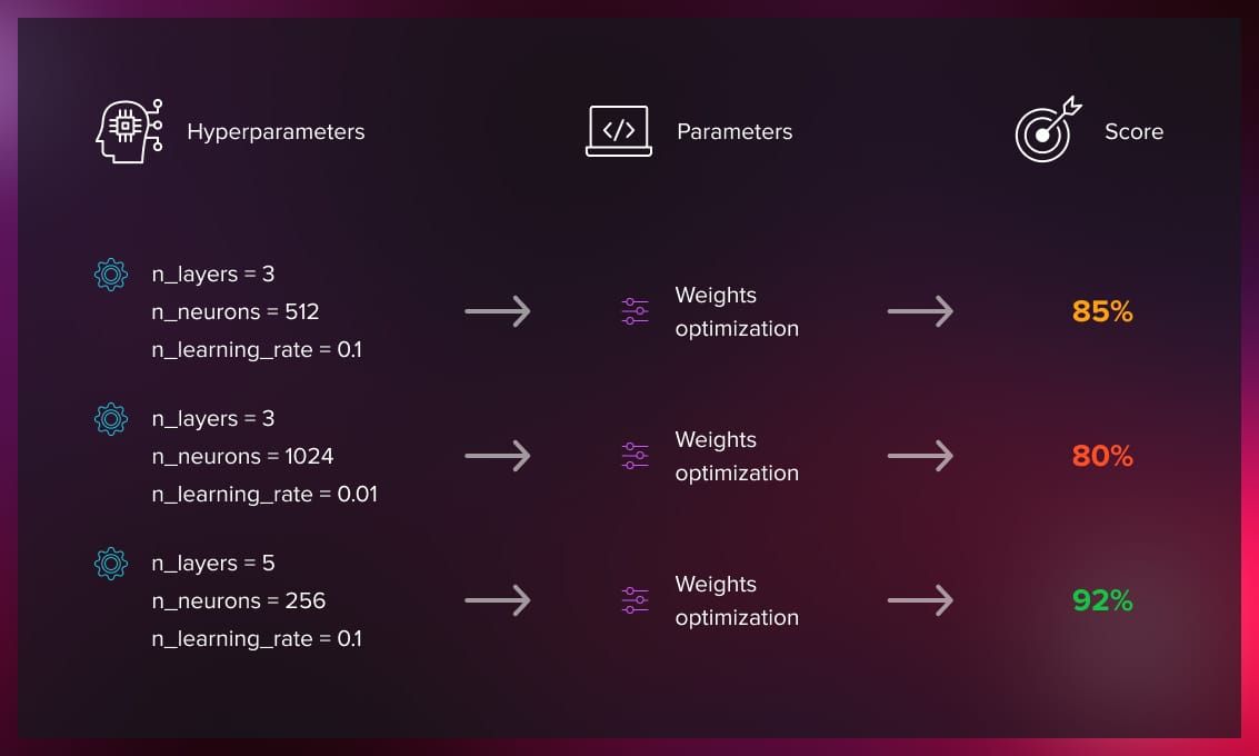
The aim of hyperparameter optimization in machine learning is to find the hyperparameters of a given ML algorithm that return the best performance as measured on a validation set.
Below you can see examples of hyperparameters for two algorithms, random forest and gradient boosting machine (GBM):
| Algorithm | Hyperparameters |
| Random forest |
|
| Gradient Boosting Machine (GBM) |
|
Read this article for a more detailed explanation of hyperparameters.
Hyperparameter optimization approaches
There are four main approaches to hyperparameter optimization.
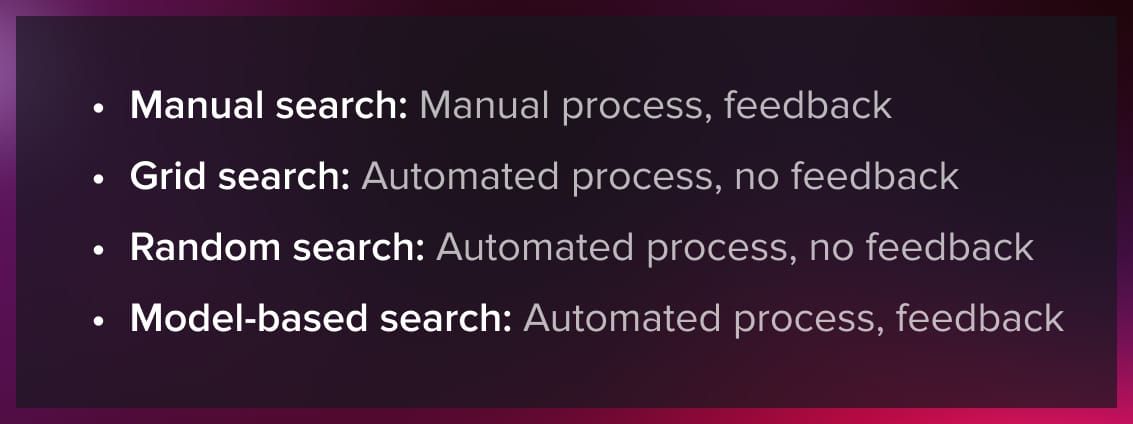
- Manual search: Hyperparameters are set manually, and evaluations of the model’s training are made iteratively.
- Grid search: This method automates the process by predefining a set of hyperparameters for systemic evaluation.
- Random search: This approach also automates the process, doing so by randomly sampling parameter values for evaluation.
- Model-based search: By combining automation and feedback, this approach adjusts hyperparameter values based on previous trial results.
Random search usually outperforms grid search in quickly finding the best settings. While manual search requires constant involvement, it benefits from learning with each attempt. Grid search operates independently without learning from past results. Random search is also automatic but doesn’t improve over time. Model-based search combines the best features of the three approaches: it’s automated and learns from each trial.
In the following sections, we’ll explore model-based search in detail.
Model-based search using Bayesian optimization
Bayesian optimization is an efficient strategy for the optimization of objective functions that are expensive to evaluate. It’s particularly useful in scenarios where the evaluation of the function takes a long time, such as tuning hyperparameters for machine learning models. Bayesian optimization works by building a probabilistic model that maps input parameters to a probability distribution of possible outcomes. This model is then used to make educated guesses about where in the parameter space the objective function might attain its optimal value.
The process involves two main components: the surrogate model and the acquisition function.
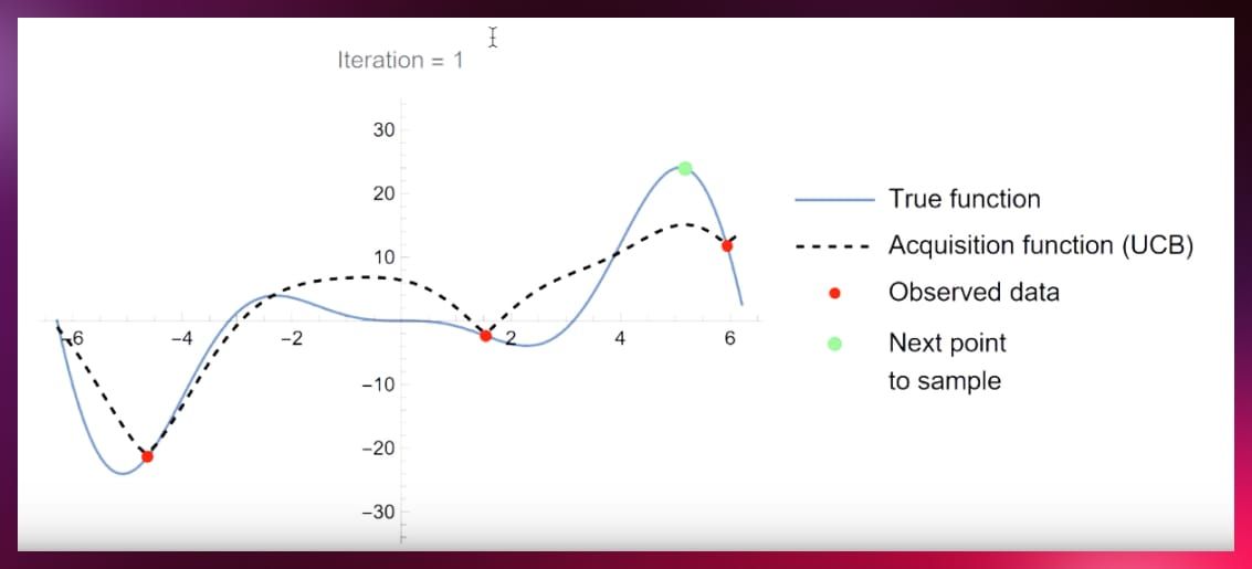
- The surrogate model, often a Gaussian process, estimates the objective function and keeps updating as new data points are evaluated. This model provides a measure of uncertainty or confidence in the predictions at unexplored points in the parameter space.
- The acquisition function uses the surrogate model’s predictions to decide which point in the parameter space should be evaluated next. It strikes a balance between exploring new areas with high uncertainty and exploiting areas known to offer promising results.
Bayesian optimization iteratively selects the next points to evaluate by optimizing the acquisition function, assesses the objective function at these points, and updates the surrogate model with the new findings. This cycle continues until a stopping criterion is met, such as a maximum number of iterations or a satisfactory level of optimization. This method is highly effective in finding the global optimum of complex functions with a relatively small number of function evaluations, making it ideal for hyperparameter tuning and other optimization tasks where function evaluations are costly.
Surrogate model
The surrogate model (SM) is a probabilistic estimator that can fit the observed data points and quantify the uncertainty of unobserved areas. So, SM is our effort to approximate the unknown black-box function f(x).
Acquisition function
The acquisition function “looks” at the SM and determines what areas in the domain of f(x) are worth exploiting and what areas are worth exploring.
Accordingly, in areas where f(x) is optimal or areas that we haven’t yet looked at, AF assumes a high value. On the contrary, in areas where f(x) is suboptimal or areas that we have already sampled from, AF’s value is small.
Example
We start by using scikit-learn to generate a binary classification dataset with 2000 samples, featuring a total of 25 features. This includes seven informative features with important hyperparameters for our binary classification task, alongside ten features that are intentionally redundant. (Though mainly set up for binary classification, this dataset is versatile enough to be adjusted for regression analyses as well.)
We then split our dataset, reserving 20% for testing purposes while the rest is used for training our model.
The next step involves optimizing the hyperparameters of a random forest model to improve its accuracy. To achieve this, we define an objective function that essentially measures how well our model performs by using the negative accuracy score. This approach allows us to turn our goal of maximizing accuracy into a problem of minimization, which fits neatly into our optimization framework. We carefully outline the search space for our model’s hyperparameters, including criteria for splitting, number of trees, maximum depth, and maximum features.
Finally, we employ the Bayesian optimization algorithm by using the fmin function, which systematically navigates through our predefined search space based on the performance feedback from our objective function.
This process is iterative, with each trial recorded to refine our search and find optimal hyperparameters setting. Through this approach, we aim to pinpoint the configuration that minimizes our objective function, thus achieving the highest possible accuracy for the random forest model on our task.
You can use sklear hyperopt to carry out your own task.
For more information on fmin and other aspects of Bayesian optimization, we recommend that you refer to this paper.
How to improve Bayesian optimization?
Two significant enhancements can substantially improve the Bayesian optimization algorithm’s efficiency.
Cold start problem
The first improvement targets the “cold start problem,” where the initial phase of the algorithm relies on randomly sampling hyperparameters to build the surrogate model. A more effective initiation strategy can significantly reduce the number of iterations needed to converge to the optimal values. This requires an approach that minimizes reliance on random sampling, aiming to start the optimization process closer to the most promising hyperparameter values.
This initial challenge is that starting points can significantly impact the time and resources required for model convergence.
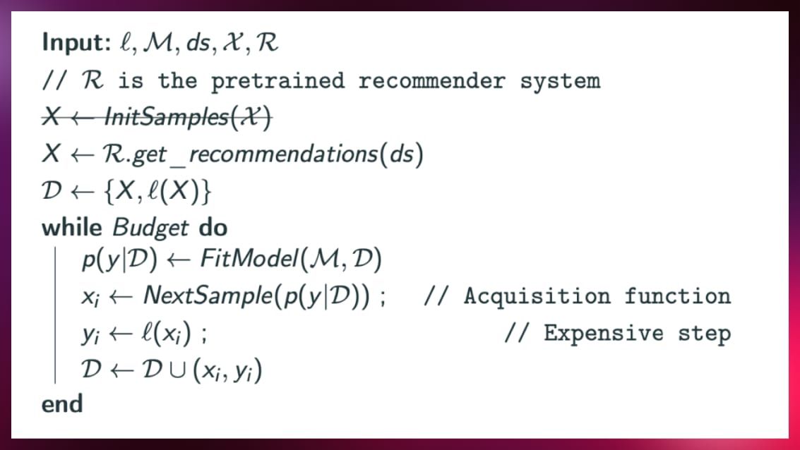
Hyperparameter recommendation system
The second improvement is the creation of a hyperparameter recommendation system. This system would function similarly to the recommendation algorithms utilized by streaming services like Netflix and YouTube, using matrix factorization techniques to suggest the most suitable hyperparameters based on past data.
To develop such a recommender system, we used offline datasets described by meta-features that reflect their characteristics, including data distributions, sample sizes, and the number of columns. By repeatedly training models on these datasets with various hyperparameters and identifying the best-performing ones, we built a large database that links dataset meta-features to their ideal hyperparameters. This knowledge base then guided the selection of hyperparameters for new datasets, enhancing the optimization process.
The hyperparameter recommendation system improves the model optimization process by analyzing the characteristics of a dataset and comparing them to a comprehensive knowledge base. It calculates meta-features, such as data distribution, sample size, and feature count, of the current dataset and identifies the most similar dataset within the knowledge base. Based on this similarity, the system recommends hyperparameters that have previously shown to be optimal for the closely matched dataset. This approach offers a collection of well-chosen initial hyperparameters, effectively tackling the “cold start” challenge. It eliminates the reliance on random sampling to begin the optimization process.
To further streamline the optimization process, we used a method that allowed us to reduce the computationally intensive task of repeatedly training models with various hyperparameters. Instead of direct training, we introduced a predictive model that estimates the performance of any given hyperparameter set. This predictive model was initially trained on a diverse collection of tasks, using an offline dataset that pairs hyperparameters with their resultant performance metrics. However, since such a dataset may not exist upfront, ensemble learning can be used to build this predictor with data from various sources, ensuring a broad and robust foundation. Upon deployment, the system was able to fine-tune this predictor using data from its early recommendations, which refined its accuracy for future hyperparameter suggestions.
Conclusion
In conclusion, the Bayesian optimization algorithm stands out as a highly effective method for hyperparameter optimization in machine learning models. By employing a probabilistic model to guide the search for the optimal set of hyperparameters, Bayesian optimization significantly reduces the number of trials needed to find an optimal solution. This not only saves time and computational resources but also enables the development of more accurate and robust machine learning models, as we have seen in the studied example.


.jpg)
.jpg)
.jpg)
.jpg)