
Developing an effective and accurate ML model to solve a problem is one of the goals of any AI project. To optimize the model, we need to tune its parameters and hyperparameters and then evaluate whether the updates result in the anticipated improvements. This requires setting up key metrics and defining a model evaluation procedure. After implementing the changes and conducting evaluation, we can determine if the performance of the ML model has improved and whether we should use the updated version.
What are hyperparameters and how do they differ from parameters?
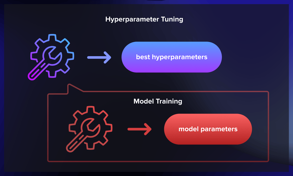
Parameters in machine learning are special coefficients or weights of the model that are selected and tuned during the training process. They are estimated by fitting the training data to the model and are subsequently used to make predictions on new data.
In contrast, hyperparameters are set before the training process. They are unique settings that govern the learning process in ML and directly impact the model parameters that an algorithm learns.
Hyperparameters can’t alter themselves while the model is in its learning or training stage, and they don’t make it into the final model. Moreover, it’s impossible to discern the values of the hyperparameters used during training just by examining the model; only the learned model parameters are evident. Examples of hyperparameters include the learning rate, the number of hidden layers in a neural network, and the regularization parameter.
What is hyperparameter tuning?
Hyperparameter tuning is the process of selecting the optimal values for the hyperparameters of a machine learning algorithm or model. It’s a critical step in machine learning model development.
Hyperparameter tuning involves finding the optimal combination of hyperparameter values that maximize a specific evaluation metric. The objective is to identify the set of hyperparameters that, when introduced to the machine learning model, yield the highest performance on unseen data or demonstrate effective generalization to new examples. By carefully adjusting these hyperparameters, we aim to enhance the model’s ability to make accurate predictions and improve its overall performance.
Key hyperparameters that can be tuned in NN include:
- Number of hidden layers in the neural network: Balancing simplicity (which ensures speed and generalization) with accurate model performance is crucial. Starting with four to six hidden layers can be a good initial strategy, and the number can be adjusted based on the requirements for the prediction accuracy.
- Number of nodes/neurons per layer: Having more neurons per layer isn’t always beneficial. While an increase can enhance performance, too many neurons may lead the network to memorize the training dataset, which could reduce accuracy when dealing with new data.
- Learning rate: This hyperparameter influences how much the model parameters are adjusted in each iteration. A lower learning rate means smaller changes to parameter estimates, implying a longer time (and more data) is required to train the model. However, a lower learning rate can also increase the likelihood of achieving minimum loss. Finding an optimal learning rate often involves experimentation and parameter fine-tuning. Techniques like learning rate schedules, where the learning rate is adjusted over time, or adaptive learning rate algorithms, such as Adam or RMSprop, are among the ones often used.
- Momentum: This hyperparameter is helpful to prevent the model from getting stuck in local minima. Mathematically, momentum can be defined as a weighted average of the gradients computed over previous iterations. By including a momentum term, the network can maintain a certain level of inertia, which helps prevent sudden changes and promotes a more stable convergence. The introduction of momentum in neural networks enhances the speed of convergence, especially when dealing with complex and high-dimensional data. Additionally, momentum contributes to the network’s ability to generalize well to unseen data by reducing overfitting. A recommended approach is to start with low momentum values and gradually increase them as needed.
What is the process of hyperparameter tuning?
Hyperparameter tuning can be performed manually or by using automated methods. While time-consuming and laborious, manual tuning offers an advantage because it provides a deeper understanding of how different hyperparameters influence the model’s performance. However, in most scenarios, it’s common to employ one of the recognized hyperparameter learning algorithms.
Hyperparameter tuning is a cyclical process involving experimentation with various combinations of parameters and their corresponding values. Typically, the process begins with specifying a key metric, such as accuracy. To prevent your model from overfitting, it’s recommended to use cross-validation techniques during the tuning process.
Several of the most widely used automated techniques today include grid search, random search, and Bayesian optimization. Let’s delve deeper into these methods.
Grid search
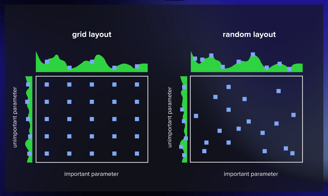
Grid search involves constructing a grid of possible discrete hyperparameter values and then training the model using all possible combinations. Your objective is to note the model’s performance for each combination and choose the set that produces the best results.
Grid search is a comprehensive technique capable of identifying the optimal hyperparameter combination. However, its major limitation is its slow pace. Fitting the model with every conceivable combination requires extensive computational resources and substantial time, which may not always be feasible or available.
Pros: The grid search method remains popular due to its straightforwardness and efficacy, especially when dealing with smaller, less intricate models.
Cons: As the method involves training individual models for various combinations of hyperparameters, making it computationally demanding. Additionally, its effectiveness is constrained by the predetermined range of possible values for each hyperparameter, potentially excluding the optimal values.
Random search
As the name suggests, random search selects hyperparameter values randomly rather than sticking to a prearranged order, as is the case with the grid search method.
In each iteration, random search tests a random assortment of hyperparameters and oversees the model’s performance. After several iterations, it presents the combination that led to the best outcome.
Random search is handy when dealing with numerous hyperparameters with relatively broad search domains. Even with discrete ranges defined, this method can still produce a reasonably effective set of combinations.
One advantage of random search is that it usually consumes less time than grid search to get a result. It also prevents the model from favoring arbitrarily picked value sets. The downside is that the resulting combination may be different from the optimal set of hyperparameters.
Pros: The ease of implementation makes random search a popular choice.
Cons: The random search method is less structured and may be less efficient in identifying the optimal set of hyperparameters, especially for larger and more complex models.
Bayesian optimization
The grid search and random search methods may not be efficient enough as they may examine numerous poor hyperparameter combinations. They fail to use insights from earlier iterations when determining the next hyperparameters to test.
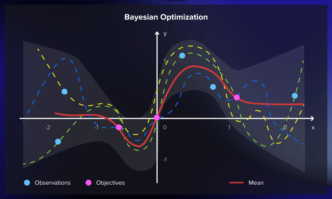
Bayesian optimization does incorporate results from previous evaluations. By deploying a probabilistic function, it determines hyperparameters that can provide the best results, usually discovering an effective combination with fewer iterations.
When the objective function to be maximized or minimized doesn’t have a known analytical representation, data scientists opt for a probabilistic model. They run a learning algorithm on a dataset and use its output to formulate the objective function. In this scenario, different hyperparameter combinations are seen as potential inputs.
The probabilistic model uses past evaluation results to estimate the probability of achieving a certain outcome with a specific set of hyperparameters. It serves as a “surrogate” for the objective function, which could, for instance, be the root-mean-square error (RMSE).
The probabilistic model’s application to the hyperparameters is computationally less demanding than the objective function. Hence, this method improves the probability model each time you run the objective function. This results in better predictions of hyperparameters, reducing the number of the objective function’s evaluations required to achieve a satisfactory result.
Surrogate models can take various forms, including Gaussian processes, random forest regression, and tree-structured Parzen estimators (TPE).
Pros: Bayesian optimization is better at identifying the optimal set of hyperparameters than random search and grid search, especially when dealing with larger and more complex models. Additionally, Bayesian optimization is particularly advantageous when the objective function is noisy or computationally expensive to evaluate.
Cons: When the search dimension significantly increases, the efficiency of Bayesian optimization substantially diminishes.
The implementation of the Bayesian optimization model can be quite complex. But this process can be simplified with the help of accessible libraries like Ray Tune.
Bayesian optimization is particularly beneficial when the objective function is resource-intensive and time-consuming. Compared to grid or random search, one limitation is that Bayesian optimization calculations must be conducted in sequence (each iteration relies on the outcome of the previous one), precluding the possibility of distributed processing. Therefore, Bayesian optimization might take longer.
What hyperparameter tuning algorithms to use?
Three different types of algorithms can be used for hyperparameter optimization.
First, we’ve got exhaustive search algorithms, which look through every possibility in the search space until they find the best hyper-parameters.
Then, there are surrogate models, which use a mathematical model to estimate which hyper-parameters will be the best.
Lastly, there are some algorithms that mix ideas from both of these categories to find the optimal hyper-parameters.
Regardless of which type of algorithm is being used, we need to define the search space beforehand and set some boundaries and prior knowledge on the hyper-parameters, such as setting a non-uniform distribution for the search. Here are several examples of algorithms specially developed for hyperparameter tuning:
Hyperband
Hyperband is a notable example of exhaustive search algorithms and can be considered an enhanced version of random search. It integrates the explore-exploit theory to optimally allocate time for each configuration.
Population-based training (PBT)
PBT is a surrogate model and represents a combination of random search and manual tuning, mostly applied to neural network models. It initiates the process by concurrently training several neural networks with randomly chosen hyperparameters. But these networks aren’t entirely autonomous.
PBT utilizes information from the collective network population to refine the hyperparameters and decide on the next set of hyperparameter values to test.
BOHB
BOHB, which is short for Bayesian Optimization and HyperBand, merges the strategies of the Hyperband algorithm and Bayesian optimization. It’s an example of a hybrid hyperparameter tuning algorithm.
Tools for automated hyperparameter optimization
Bayesian-optimization library
The bayesian-optimization library streamlines the optimization of black box functions, which may be expensive or time-consuming to evaluate. This is achieved by iteratively constructing a probabilistic surrogate model of the objective function, which is updated with each subsequent evaluation. The algorithm then makes informed decisions about the next point to evaluate based on this surrogate model. It achieves a balance between exploration (trying out new regions) and exploitation (concentrating on promising areas).
The process involves the following actions:
- It optimizes these functions through the creation of a Gaussian process.
- The bayesian-optimization library maintains a balance between exploration within the search space and the exploitation of results derived from earlier iterations.
- It offers the ability to dynamically adjust the problem’s boundaries, enhancing convergence.
An additional noteworthy feature is the incorporation of the observer pattern. The optimization progress recorded as a JSON object can be reloaded later to initiate a new optimization. This capability facilitates the execution of partial searches that can then be continued at a later stage.
Scikit-optimize (Scopt)
When dealing with a significant number of parameters, the base algorithms such as grid search and random search offered by the widely-used scikit-learn toolkit are not always efficient. An alternative would be to utilize the scikit-optimize library (also known as skopt), which employs a Bayesian optimization strategy.
Skopt can serve as a direct replacement for the original GridSearchCV optimizer in scikit-learn. It supports multiple models with varying search spaces and number of evaluations to be optimized per model class.
Moreover, Skopt provides tools for comparing and visualizing the interim results of different optimization algorithms, making it a valuable addition to the standard scikit-learn modeling workflow. However, one notable limitation is its relatively narrow focus, as it does not include other ML frameworks.
Hyperopt
Hyperopt is a versatile, distributed library designed for hyperparameter optimization. Hyperopt enhances the optimization process by distributing the search across parallel and distributed computing resources. This approach allows for efficient exploration of the hyperparameter space across multiple machines, which proves especially useful for large-scale experiments or computationally intensive tasks. By accelerating the process in this manner, Hyperopt has become an invaluable tool for tuning models. It currently supports three optimization techniques:
- Random search
- Tree-Structured Parzen Estimators (TPEs)
- Adaptive TPEs
One of Hyperopt’s benefits is its ability to optionally distribute its optimization process through Apache Spark or MongoDB clusters, which could also be a concern.
Hyperopt is notably adaptable, boasting seamless integration with:
- Scikit-learn, via Hyperopt-sklearn
- Neural networks, via Hyperopt-nnet
- Keras, through Hyperas
- Theano’s convolutional networks, using Hyperopt-convnet
With these extensions, Hyperopt offers a broad spectrum of potential applications.
Optuna
Optuna uses the define-by-run user API. Rather than performing calculations instantly, the process dynamically constructs the hyperparameter search spaces as it unfolds. This approach offers benefits including time and resource efficiency, scalability, integration with popular libraries, visualization capabilities, and features for reproducibility.
The search techniques implemented by Optuna include:
- Traditional grid/random searches
- Tree-Structured Parzen Estimators (TPEs)
- Partially fixed hyperparameters
- A quasi-Monte Carlo sampling algorithm
Additionally, Optuna incorporates pruning algorithms that help to cease the exploration of non-promising branches within the search space.
Optuna can parallelize optimization tasks by integrating with relational databases such as MySQL. It also provides a visualization of the optimization history and a Web dashboard.
Optuna works well with the PyTorch and FastAI ML frameworks but isn’t integrated with other commonly used ML frameworks, which could be a limitation.
Ray Tune
The Ray Tune (ray) framework offers a scalable suite of utilities for machine learning, addressing three primary applications:
- Scaling machine learning workloads: Ray Tune features libraries for processing data, training models, and reinforcement learning (among others) in a distributed manner.
- Constructing distributed applications: With Ray Tune’s parallelization API, there’s no need to adjust your code to execute it on a cluster of machines.
- Deploying large-scale workloads: Ray Tune’s cluster manager is compatible with Kubernetes, YARN, and Slurm clusters, allowing deployment on major public cloud platforms.
Ray Tune excels in distributed and parallel execution scenarios, while Optuna focuses on efficient sequential optimization with a range of specialized search algorithms. The framework provides hyperparameter optimization capabilities through integration with several popular libraries, such as:
- Bayesian-optimization
- Scikit-optimize
- Hyperopt
- Optuna
Moreover, Ray Tune supports all major machine learning modeling frameworks, including PyTorch, TensorFlow, scikit-learn, Keras, and XGBoost. Ray Tune is part of an extensive ecosystem of ML/AI tools, including spaCy, Hugging Face, Ludwig, and Dask.
Watch this video to find out about deep learning hyperparameter tuning in Python, TensorFlow & Keras.
Model evaluation
Evaluation is a crucial step in assessment of the performance of a machine learning model. Accuracy, precision, recall, and the F1 score are used to identify efficiency and recognize critical weaknesses and generalization errors.
There are two main approaches for model evaluation: hold-out and cross-validation. These methods involve using a separate test set the model has not been exposed to during training, allowing for a reliable performance assessment.
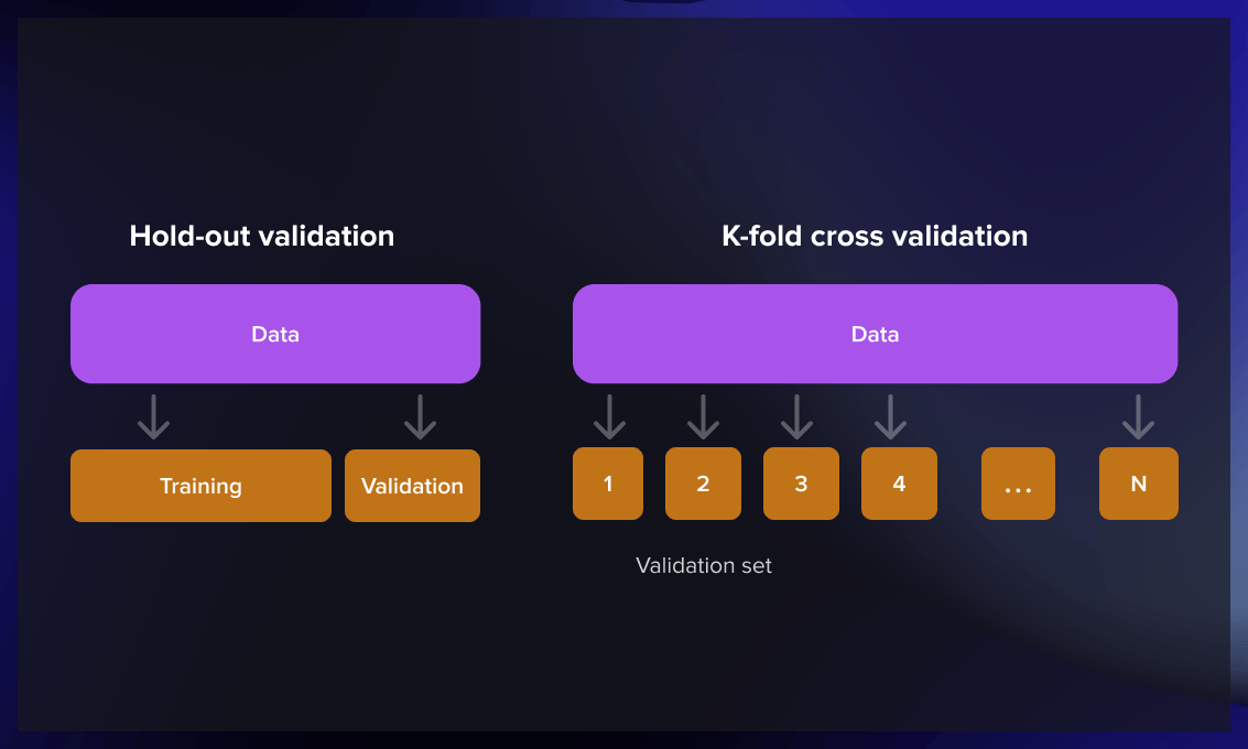
Hold-out
The hold-out method works by splitting a large dataset into three subsets at random:
- The training set is used to build predictive models.
- The validation set is employed to evaluate the model created during the training phase. It serves to fine-tune the model’s parameters and determine the most effective model. However, not every ML algorithm requires a validation set.
- The test set (unseen data) is used to predict the expected future performance of a model. If a model performs significantly better on the training set than the test set, it is likely overfit.
Cross-validation
Cross-validation is used when there is a limited amount of available data and an objective estimation of model performance is necessary. The k-fold cross-validation method divides the data into k equally sized subsets. A model is then built k times, each time excluding one of the subsets from training and using it as a test set. When k equals the sample size, this approach is called “leave-one-out.”
Metrics for model evaluation
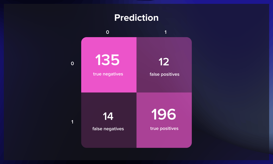
When it comes to model assessment, there are four possible outcomes.
- True positives – when an observation is correctly predicted as belonging to a specific class.
- True negatives – when the prediction accurately states that an observation doesn’t belong to a given class.
- False positives – when an observation is incorrectly assigned to a class to which it doesn’t belong.
- False negatives – when the prediction inaccurately suggests that an observation doesn’t belong to a particular class when in fact, it does.
These four types of outcomes are usually visualized with the help of a confusion matrix.
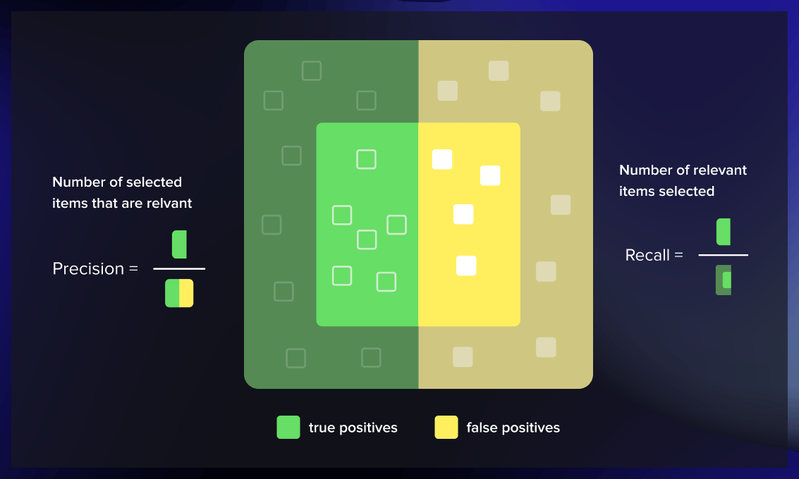
The key metrics for evaluating a classification model are accuracy, precision, and recall.
Accuracy is the proportion of correct predictions made on the test data. It can be computed by dividing the number of accurate predictions by the total number of predictions.
Precision calculates the ratio of relevant instances (true positives) over all the cases predicted as belonging to a specific class.
Recall measures the proportion of instances predicted to belong to a particular class out of all the instances that actually belong to that class.
Precision and recall are especially important when addressing issues with imbalanced class distributions. Take, for instance, the creation of a classification algorithm aimed at identifying a disease that affects a mere 1% of the population. If the model is designed to consistently predict that individuals do not have the condition, the resulting model would have an accuracy rate of 99%, but it would be entirely ineffective.
Analyzing this inept model’s recall would expose its performance’s shortcomings. In this scenario, recall ensures that the model identifies those with the disease. On the other hand, precision safeguards against the model wrongly labeling healthy individuals as having the disease. A model that inaccurately diagnoses someone with a severe illness, like cancer, would be problematic. Equally dangerous is a model that misses a genuine case of the disease. Hence, assessing both precision and recall is crucial when gauging a model’s effectiveness.
Most common mistakes with hyperparameter tuning
Correct implementation is key to unlocking the full potential of your model through hyperparameter optimization. However, data scientists should be aware of and avoid certain pitfalls to achieve successful hyperparameter tuning.
- Trusting the defaults: Relying on default hyperparameters can be inappropriate for your specific problem. The solution is to execute hyperparameter optimization to find the best values for your model.
- Using the wrong metric: Optimizing based on the wrong metric can lead to misleading results. Balancing multiple metrics or exploring different solutions can help create a better evaluation criterion.
- Overfitting: It occurs when a model performs well during training but poorly on new data. Techniques like cross-validation help prevent overfitting and ensure better generalization.
Conclusion
Hyperparameter tuning is an essential aspect of training and optimizing machine learning models. This iterative process involves selecting and refining the settings of the learning algorithm that will impact the model’s performance, such as learning rate, epoch number, and regularization parameters. Tuning can be performed manually, using a grid search, a random search, or through automated methods like Bayesian optimization.
The selection of hyperparameters can significantly influence the model’s ability to learn effectively, directly affecting both the training speed and the model’s predictive accuracy. The best hyperparameters cannot be known a priori, as they depend on the specific dataset and problem at hand, making hyperparameter tuning a crucial step in the machine learning pipeline.

.jpg)
.jpg)