
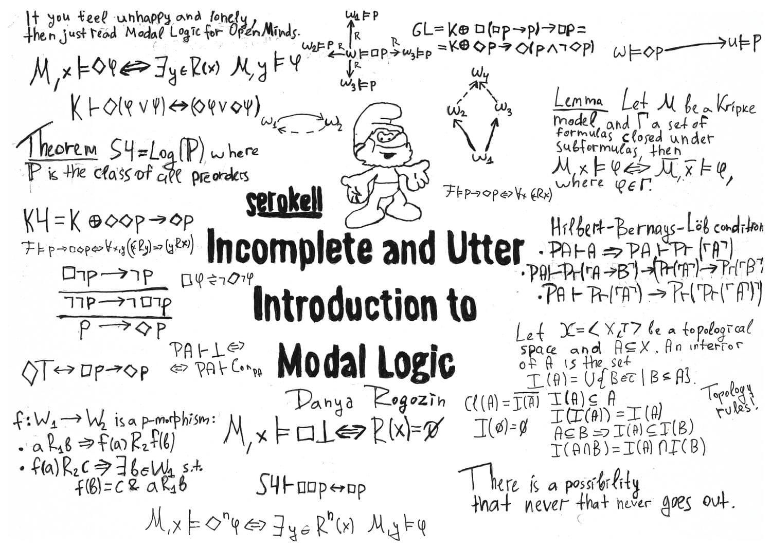
Foreword
Modal logic is one of the most popular branches of mathematical logic. Modal logic covers such areas of human knowledge as mathematics (especially, topology and graph theory), computer science, linguistics, artificial intelligence, and philosophy. Moreover, modal logic in itself still attracts by its mathematical beauty. We would like to introduce the reader to modal logic, fundamental technical tools, and connections with other disciplines. Our introduction is not so comprehensive indeed, the title is an allusion to the wonderful book by Stephen Fry.
History and background
The grandfather of modal logic is the 17th-century German mathematician and philosopher Gottfried Leibniz, one of the founders of calculus and mechanics.
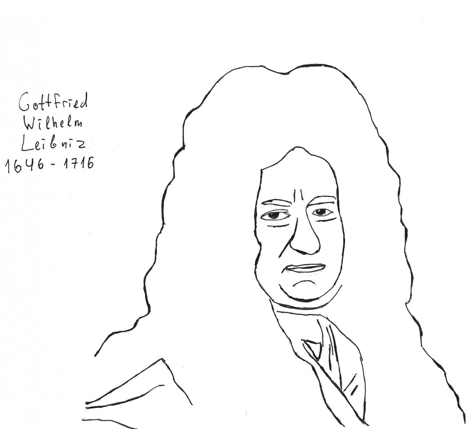
From his point of view, there are two kinds of truth. The statement is called necessarily true if it’s true for any state of affair. Note that, one also has possibly true statements. That is, such statements that could be false, other things being equal. For instance, the proposition “sir Winston Churchill was a prime minister of Great Britain in 1940” is possibly true. As we know, Edward Wood, 1st Earl of Halifax, also could be a prime minister at the same time. Of course, one may provide any other example from the history of the United Kingdom and all of them would be valid to the same degree. In other words, any factual statement might be possibly true since “the trueness” of any factual statement depends strongly on circumstances and external factors. The example of a statement which is necessarily true is , where signs , , and are understood in the usual sense.
Modal logic became a part of contemporary logic at the beginning of the 20th century. In the 1910s, Clarence Lewis, American philosopher, was the first who proposed to extend the language of classical logic with two modal connectives and .
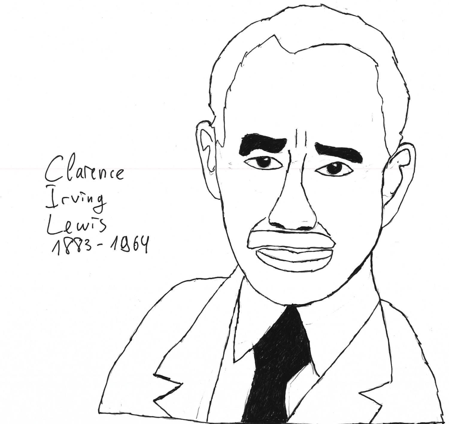
Informally, one may read as is necessary. has a dual interpretation as is possible. Lewis sought to analyse the notion of necessity from a logical point of view. Thus, modalities in mathematical logic arose initially as a tool for philosophical issue analysis. Lewis understood those modalities intuitively rather than formally. In other words, modal operators had no mathematically valid semantical interpretation.
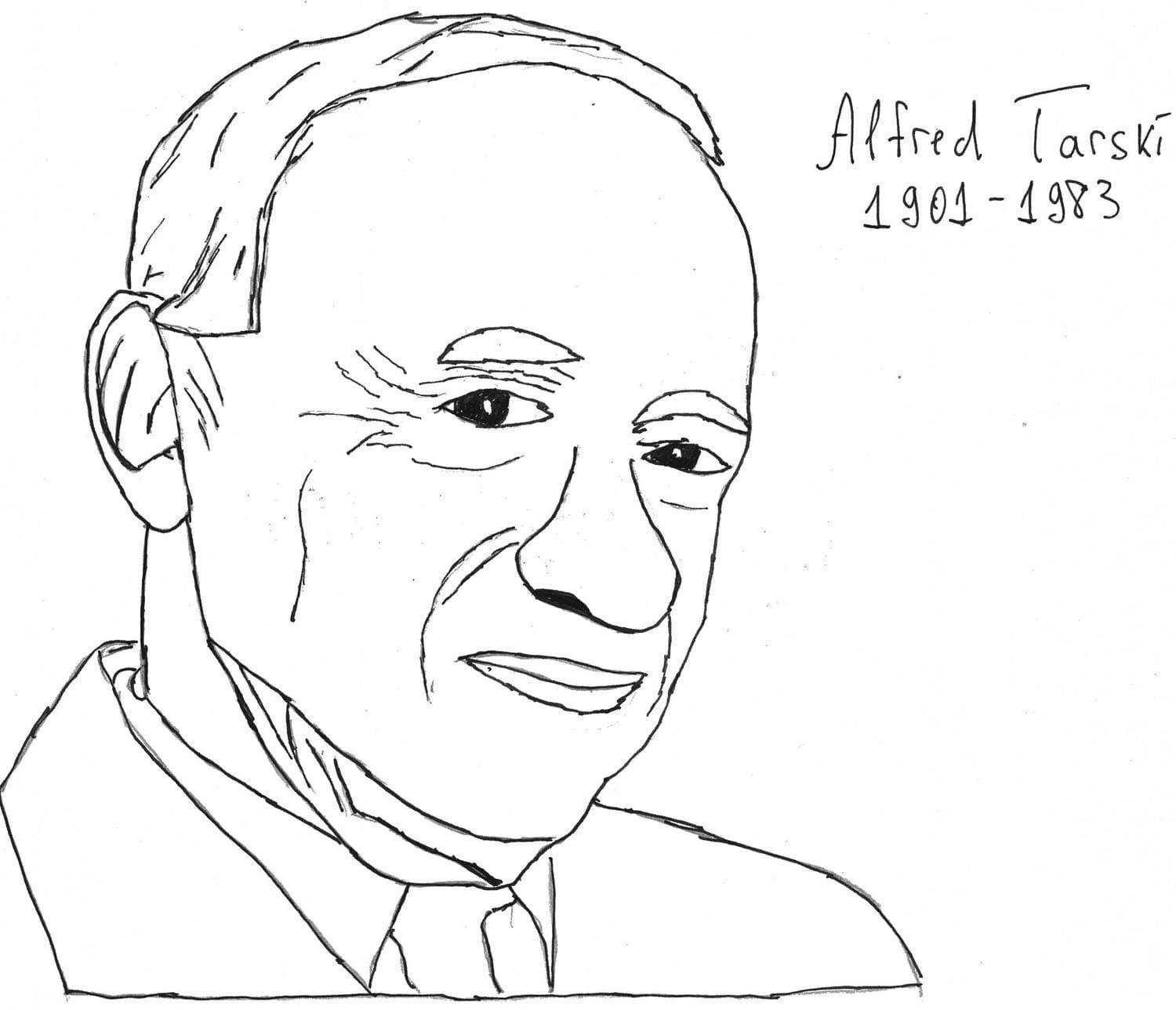
In the year 1944, Alfred Tarski and John McKinsey wrote a paper called The Algebra of Topology. In this work, the strong connection between modal logic and topological and metric spaces was established. Historically, topological semantics is the very first mathematical semantics of modal logic. Those results marked the beginning of a separate branch of modal logic that studies the topological aspects of modalities.
In the 1950s and 1960s, Saul Kripke formulated relational semantics for modal logic. Note that we will mostly consider Kripke semantics in this post.
Later, in the 1970s, such mathematicians as Dov Gabbay, Krister Segerberg, Robert Goldblatt, S. K. Thomason, Henrik Sahlqvist, Johan van Benthem provided the set of technical tools to investigate systems of modal logic much more deeply and precisely. So, modal logic continues its development in the direction that was established by these researchers.
Let us briefly overview some areas of modal logic use.
Topology and graphs
Modal logic provides a compact and laconic language to characterise some properties of directed graphs and topological spaces. In this blog post, we study Kripke frames as the underlying structures. Without loss of generality, one may think of Kripke frames as directed graphs. It means that formal definitions of a Kripke frame and a directed graph are precisely the same. Here, modal language is a powerful tool in representing first-order adjacency properties. We realise the fact that not every reader has a background in first-order logic. In order to keep the post self-contained, we remind the required notions from first-order logic to describe this connection quite clearly.
As we will see, modal logic is strongly connected with binary relations through Kripke frames. The properties of binary relation in a Kripke frame are mostly first-order. We consider examples of first-order relation properties expressed in modal language. Moreover, we formulate and discuss the famous Salqvist’s theorem that connects modal formulas of the special kind with binary relation properties that are first-order definable. Anyway, in such a perspective, one may consider modal logic as a logic of directed graphs since there is no formal difference between a binary relation and edges in a graph. That is, one may use modal logic in directed graph characterisation in a limited way.
You may draw any directed graph you prefer on a plane. A graph is a combinatorial object rather than a geometrical one. A topological space is closer to geometry. Although, there’s a topological way of graph consideration, however. We also discuss how exactly modal logic has a topological interpretation. In the author’s opinion, topological and geometrical aspects of modal logic are one of the most astonishing and beautiful.
It is a well-known result proved by Alfred Tarski and John McKinsey that the modal logic is the logic of all topological spaces. Similarly to directed graphs, modal logic might be used in classifying topological spaces and other spatial constructions in a restricted way. We will discuss the topological and spatial aspects of modal logic in the second part.
The foundations of mathematics
The foundation of mathematics is the branch of mathematical logic that studies miscellaneous metamathematical issues. In mathematics, we often consider some abstract structure and formulate a theory based on some list axioms that describe primitive properties of considered constructions. The examples are group theory, elementary geometry, graph theory, arithmetics, etc.
In metamathematics, we are interested in what a mathematical theory is in itself. That is, metamathematics arose at the beginning of the previous century to answer philosophical questions mathematically. The main interest was to prove the consistency of formal arithmetics with purely formal methods. As it’s well known, Gödel’s famous incompleteness theorems place limits the formal proof of arithmetics consistency within arithmetics itself.
However, modal logic also allows one to study the properties of provability in formal arithmetical theories. Moreover, the second Gödel’s incompleteness theorem has a purely modal formulation! We discuss that topic in more detail in the follow-up of the series.
Basic definitions and constructions
Modal language
Let us define the modal language. That’s the starting point for every logic which we take into consideration. In our case, a modal language is a grammar according to rules of which we write logical formulas enriched with modalities. Let be a countably infinite set of propositional variables, or atomic propositions, or propositional letters. Informally, a propositional variable ranges over such atomic statements as “it is raining” or something like that.
A modal language as the set of modal formulas is defined as follows:
- Any is a formula.
- If is a formula, then is a formula.
- If and are formulas, then is formula, where .
- If is a formula, then is a formula.
Note that the possibility operator is expressed as = . In our approach, the statement is possibly true if it’s false that necessiation of is true. Also, one may introduce as the primitive one, that is .
Also, it is useful to have constants and that we define as and correspondingly.
As we said, a modal language extends the classical one. One may ask how we can read . Here are several ways to understand this modal connective:
- as is necessary. This is historically the very first way of the modal connective reading. Dually, one may read as is possible. Modalities of this kind are alethic modalities.
- as it is known that . In this case, we call an epistemic modality.
- as is a statement provable in formal arithmetics.
- as an interior in a topological space. Here, we call such modality a topological one.
- as there will be always in the future, a temporal modality, in other words.
We will discuss items 3-5 in the next part of the series as promised.
Modal logic
We defined the syntax of modal logic above. But syntax doesn’t provide logic, only grammar. In logic, one has inference rules and the definition of proof. We also want to know what kind of modal statements we need to prove basically. Firstly, let us describe a more basic notion like normal modal logic.
By normal modal logic, we mean a set of modal formulas that contains all Boolean tautologies; -axiom (named after Kripke) and closed under the following three inference rules:
- If and , then (Modus ponens). That is the basic logical rule that allows you to get a consequence from an implication if you have a premise.
- If , then (Necessiation rule). If belongs to a logic, then belongs to too. Informally, if is provable, then is necessary.
- If , then . If formula with variable belongs to a logic, then its instances belong to the same logic. Here, the instance of the formula is the result of a substitution of another formula instead of a variable. In other words, any normal modal logic is closed under substitution.
The fact that any normal modal logic contains all Boolean tautologies tell us that modal logic extends the classical one. Literally, the Kripke axiom -axiom denotes that distributes over implication. Such an explanation doesn’t help us so much, indeed. It’s quite convenient to read this axiom in terms of necessity. Then, if the implication is necessary and the premise is necessary, then the consequence is also necessary. For instance, it is necessary that if the number is divided by four then this number is divided by two. Then, if it is necessary that the number is divided by four, then it is necessary that it’s divided by two.
Of course, within the natural language that we use in everyday speech the last two sentences sound quite monotonous, but we merely illustrated how this logical form works by example. In such a situation, it’s crucially important to follow the formal structure even if this structure looks wordy and counterintuitive. Of course, this sometimes runs counter to our preferences in linguistic aesthetics, although structure following allows analysing modal sentences much more precisely.
If we take into consideration some logical system represented by axioms and inference rules, then one needs to determine what derivation is in an arbitrary normal modal logic. A derivation of formula in normal modal logic is a sequence of formulas, each element of which is either axiom or some formula obtained from the previous ones via inference rules. The last element of such a sequence is a formula itself.
Here is an example of derivation in normal modal logic:
- Boolean tautology
- Necessiation rule
- -axiom.
- Modus ponens, (2), (3)
- -axiom
- Transitivity of implication, (4), (5)
- The instance of a Boolean tautology
- Modus ponens, (6), (7)
We leave the converse implication as an exercise to the reader.
The minimal normal modal logic is defined via the following list of axioms and inference rules:
- ,
- ,
- Inference rules: Modus Ponens, Necessiation, Substitution.
The axioms (1)-(8) are exactly axioms of the usual classical propositional logic that axiomatise the set of Boolean tautologies together with Modus Ponens and Substitution rule. The axiom (9) is a Kripke axiom . One may also claim that is the smallest normal modal logic. In the definition of normal modal logic, we just require that the set of formulas should contain Boolean tautologies, etc. By the way, there might be something different from the required list of formulas. For instance, the set of all formulas is also a normal modal logic, the trivial one. The minimal normal modal logic is a normal modal logic that contains only Boolean tautologies, -axiom and closed under the inference rules, no less no more. The logic is the underlying logic for us. Other modal logics are solely extensions of . Note that modal logic is not needed to be a normal one. Weaker modal logics are studied via so-called neighbourhood semantics that we drop in our introductory post.
Kripke semantics
We have defined the syntax of the modal logic above introducing the grammar of a modal language. Let us define Kripke frames and models to have the truth definition in modal logic.
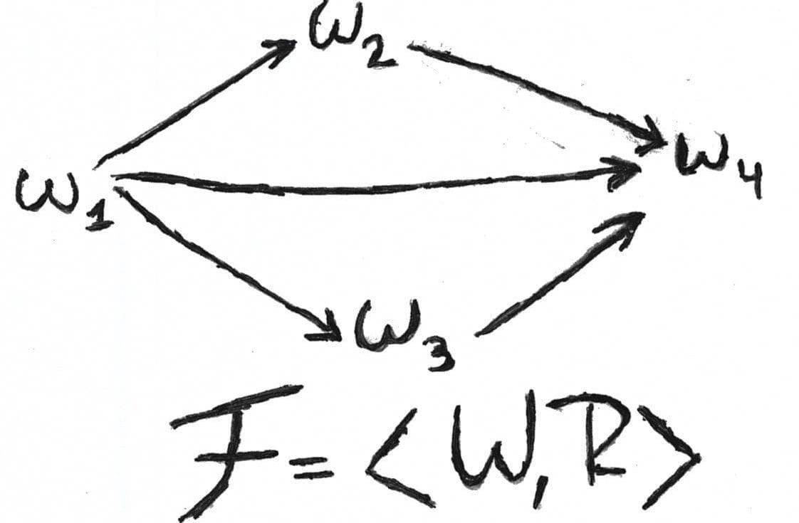
Definition A Kripke frame is a pair , where is a non-empty set, a set of so-called possible worlds, informally. Note that we will call an element of a world or a point. World and point are synonyms for us. is a binary relation on . For example, the set with strict order relation is a Kripke frame. Moreover, any directed graph might be considered as a Kripke frame, where the set of vertices is a set of possible worlds and the set of edges is a binary relation.
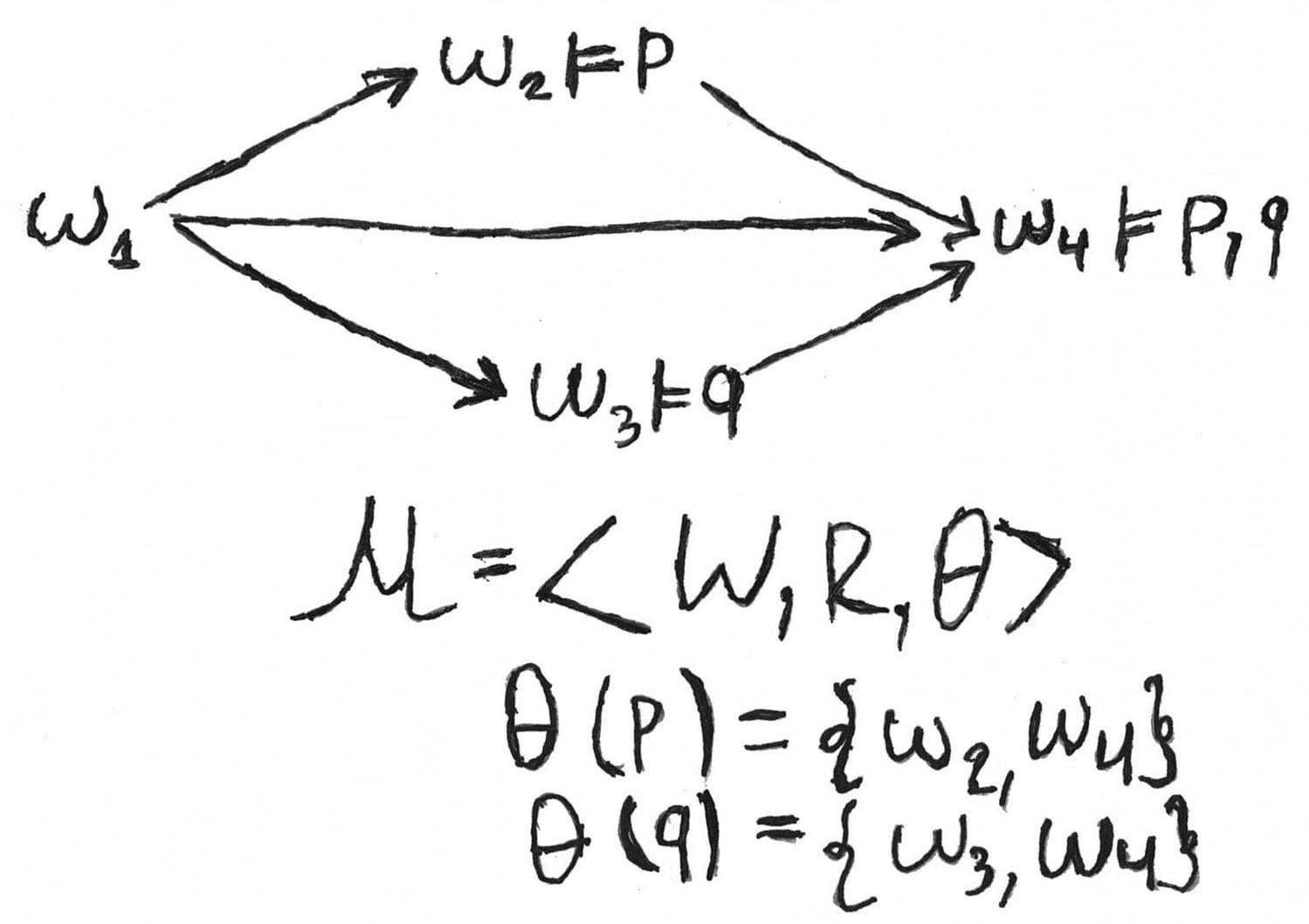
Definition A Kripke model is a pair , where is a Kripke frame and is a valuation function that maps any proposition variable to some subset of possible words. Informally, we should match any atomic statement with corresponding states of affairs in which this atomic statement is true. For complex formulas, we introduce the truth definition inductively. We denote this relation as that should be readen as “in model , in world the statement is true”.
- iff
- , that is, there is no point in which false could be true.
- iff implies
- iff for all such that ,
It is not so difficult to obtain the truth conditions for other connectives. One needs to keep in mind that the other Boolean connectives are introduced via implication and bottom as
We also know that , so the truth definition for is the following one:
iff there exists such that and .
There are a lot of examples of Kripke models, indeed. Here, we refer the reader to the book Modal Logic of Open Minds by Johan van Benthem to study miscellaneous cases in depth. Let us consider briefly the following graph as a Kripke frame with the valuation map :
Also, we will use the following notions:
- iff for each . That is, a formula is true in a Kripke model if and only if it’s true in each possible world
- iff for each valuation and for all , . One should read as is valid in a frame In other words, a formula is true in a Kripke frame if and only if it’s true in every Kripke model on this frame as an underlying one.
- , where is a Kripke frame. We will call the set the logic of frame
- Let be a class of Kripke frames, then . More simply, the logic of class is a set of formulas each of which is true in every Kripke frame that belongs to this class.
In logic, we often require that any true formula should be provable. If some logic satisfies this requirement, then we call that the logic is complete. Here, a modal logic is a Kripke complete if and only if there exists some class of Kripke frames such that . That is, any valid formula in this class of frames is provable in .
So, we’re going to solve the following issue. What’s the most general logic which is valid in an arbitrary Kripke frame? In other words, we are going to characterise the logic of all possible Kripke frames. We defined above what minimal normal modal logic is. One may show that this logic is the logic of all Kripke frames:
Theorem
, where is the class of all Kripke frames.
The left inclusion called soundness is more or less obvious. The soundness theorem claims that the logic of all Kripke frames is the normal modal one. We will prove only that any formula provable in is valid in any Kripke frame and show that is closed under substitution, where is an arbitrary Kripke frame.
Let us show that the normality axiom is valid in an arbitrary Kripke frame.
Let be a Kripke frame and a valuation map. So, we have a Kripke model . Let and . Let , then and by the truth definition for . So , so far as Modus Ponens holds in every Kripke model. Thus, .
Now we show that is closed under substitution. We provide only a sketch since the full proof is quite technical.
Let be a valuation and a Kripke model. Let us put , the set of all points in a Kripke model, where the formula is true. Let and let be an arbitrary formula. We build a Kripke model such that . Then, one may show by induction that .
The right inclusion () called completeness is quite non-trivial, one needs to build the so-called canonical model. We haven’t defined what a canonical frame and model are. The idea of a canonical frame is that an observed logic itself forms a Kripke frame (and Kripke model too). Canonical frames and models often allow us to prove the fact that some normal modal logic is complete with respect to some class of Kripke frames. We provide only the main proof sketch. The following construction is very and very abstract, but sometimes one has to be patient to produce fruits.
Let be a set of formulas and a normal modal logic. is -inconsistent, if there exist some formulas such that . That is, the set of formulas is -inconsistent, if there exists a finite subset such that negation of its conjuction is provable in an observed logic. is -consistent, if is not inconsistent.
A -consistent set is maximal if it doesn’t have any non-trivial extensions. In other words, if is a subset of , where is a -consistent, then .
Now we are ready to define a canonical frame. Let be a normal modal logic, then a canonical frame is a pair , where is the set of all maximal -consistent set. is a canonical relation such that:
. That is, any boxed formula from can be unboxed in .
A canonical model is a canonical frame equipped with the canonical valuation . This valuation maps each variable to set of all maximal -consistent sets that contain a given variable.
Here comes the theorem:
Theorem
- , i.e., the truth definition is generated by membership to some maximal consistent set.
- is provable in iff , i.e. any formula is provable iff it is true at every point of a canonical model.
- If , then is provable in , i.e. any formula that valid in a canonical frame is provable.
The completeness theorem for is a simple corollary from the theorem above. Any formula that provable in is valid in every frame. If it is valid in every frame, then it is also valid in the canonical frame. Thus, a formula provable in . That’s it. The construction above allow us to claim that any formula that valid in all possible Kripke frames is provable in . The reader might read the complete proof here.
Modal logic meet first-order logic
As we told above, modal logic is strictly connected with first-order logic. First-order logic extends classical logic with quantifiers as follows. Classical propositional logic deals with statements and the ways of their combinations with such connectives as a conjunction, disjunction, negation, and implication. For example, if Neil Robertson will make a maximum 147 break, then he will win the current frame (a snooker frame, not Kripke frame). This statement has the form . denotes Neil Robertson will make a maximum 147 break. denotes he will win the current frame. In first-order logic, one may analyse formally universal and existential statements which tell about properties of objects.
More strictly, we add to the list of logical connectives quantifiers (for all …) and (there exists …). We extended the set of connectives, so one needs to redefine the notion of formula. Suppose also we have a countably infinite set of relation symbols (or letters) of arbitrary finite arity. We well denote them as . Also one has a countably infinite set of individual variables .
The notion of formula with such set of predicate symbols:
- If are variables and is a relation symbol of an arity , then is a formula
- is a formula
- If are formulas, then is a formula
- If is a variable and is a formula
The other connectives and quantifiers are expressed as follows:
Note that there is a need to distinguish free and bound variables in a first-order formula. A variable is bounded if it’s captured by a quantifier. Otherwise, a variable is called free. For instance, the variable is bounded in the formula . One may read this formula, for instance, as there is exists a point such that lies between points and . Variables and are free in this formula since there are no quantifiers that bound them.
Now we would like to realise what truth for a first-order formula is. Unfortunately, we don’t have truth tables with 0 and 1 as in classical propositional logic. The definition of truth for the first-order case is much more sophisticated. An interpretation of the first-order language (as the infinite set of relation symbols) is a pair , where is a non-empty set (a domain) and is an interpretation function. maps every relation letter of an arity to the function of type , i.e., some -ary predicate on a domain . To define truth conditions for first-order formulas, we suppose that we have an arbitrary variable assignment function such that maps every variable to some element of our domain . An interpretation and variable assignment give us a first-order model, the definition of truth is the following one:
- for each
Note that the truth definition for existential formulas might be expressed as follows: for some .
A first-order formula is satisfiable if it’s true in some model and it’s valid if it’s true in every interpretation.
We use in the same sense as in Kripke models, but with the index to distinguish both relations that denoted equally.
Let us comment on the conditions briefly. The first condition is the underlying one. As we said above any -ary relation symbol maps to -ary relation on observed domain, that is, -ary truth function . On the other hand, any variable (which should be free, indeed) maps to some element of a domain. After that, we apply the obtained truth function to the result of the variable assignment. We obviously require that an elementary formula is true in the model if the result of that application equals . The last fact mean that a predicate is true on elements .
For example, suppose we have a ternary relation symbol such that we have interpret as lies between points and . Suppose also that our domain is the real line . We map our ternary symbol to the truth function such that if and only if and . We also define the variable assignment as , , and .
It is clear that in the model on real numbers the formula is true since . The last equation follows from the obvious fact that .
The items 2 and 3 are agreed with our understanding of what false and implication are. The last condition is the truth condition for quantified formulas. This condition describes our intuition about the circumstance when a universal statement is true. Let us consider an example. Let us assume that we want to read the formula as has a father. Our domain is the set of all people who have ever lived on the planet. Then the statement is true since every human has a father, as the reader already knows even regardless of this post.
Now let us return to modal logic and Kripke models. Let us take a look at truth defitions for and one more time:
- , i.e., a formula is true at the point , if there exists -successor of , namely, such that a formula is true.
- , i.e., a formula is true at the point , if at every -successor of a formula is true.
In those explanations, we used first-order quantifiers over points in Kripke models informally. But we may build the bridge between Kripke models and first-order one more precisely. Let us assume that we have the following list of predicate and relation symbols:
- A binary relation symbols
- A countable infinite set of unary predicate letters , where
The translation from modal formulas to first-order ones is defined inductively
- , where is a variable
The translation for diamonds is the following one:
In other words, every modal formula has its first-order counterpart, a formula with one free variable .
The reader can see that we just mapped modalised formulas the first-order one with respect to their truth definition. But there’s the question: is the truth of formula really preserved with such a translation? Here is the lemma:
Lemma
Let be a Kripke model and , then if and only if .
Here is the first-order model such that its domain is , and interpretation for the predicate letter is agreed with the relation on an observed Kripke frame. An interpretation of unary predicate letters is agreed with the evaluation in a Kripke model as follows. if and only if . Here is a propositional variable with the same index . In other words, those unary predicate letters allow us to encode an evaluation via the first-order language.
The lemma claims that a modal formula is true at some point if only if its translation (in which a point is a parameter) in the first-order language is true in the corresponding model and, hence, satisfiable. That is, one has a bridge between truth in a Kripke modal and first-order satisfiability. If a formula is true in some model at some point, it doesn’t imply its provability in the minimal normal modal logic. We would like to connect provability in and in first-order predicate calculus. Here is the theorem proved by Johan van Benthem in the 1970s:
Theorem
A formula is provable in iff and only the universal closure of its standard translation is provable in the first-order predicate calculus.
That is, there’s an embedding of to first-order logic. The lemma and the theorem above gives more precise meaning of the analogy between modalities and quantifiers which looks informal prima facie.
Modal formulas and the corresponding properties of Kripke frames.
Modal formulas are closely connected with the special properties of relations on Kripke frames. We mean a modal formula is able to express the condition on a relation in a Kripke frame. Let us consider a simple example.
Suppose we have a set with transitive relation . It means that for all , if and , then . Let us show that formula is valid on frame if and only if this frame is transitive. For simplicity, we will use the equivalent form written in diamonds: . It is very easy to show that these formulas are equivalent to each other:
Lemma
Let , then iff is transitive.
Let be a transitive frame, be a valutation and . So, we have a Kripke model . Suppose . We need to show that . If , then there exists such that and . But, there exists such that and . Well, we have and , so we also have by transitivity. Hence, . Consequently, .
The converse implication is harder a little bit. Let be a Kripke frame such that , that is, this formula is true for each valuation map. Let such that and . Let us show that .
Suppose, we have the valuation such that . So, . On the other hand, , so . But we have only one point, where is true, . So, .
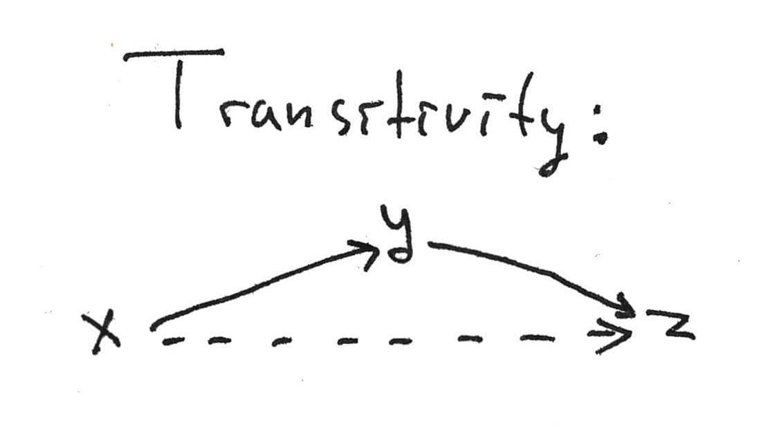
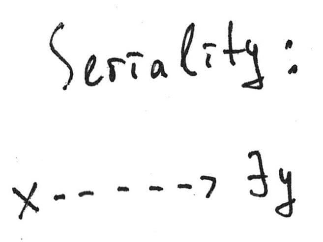
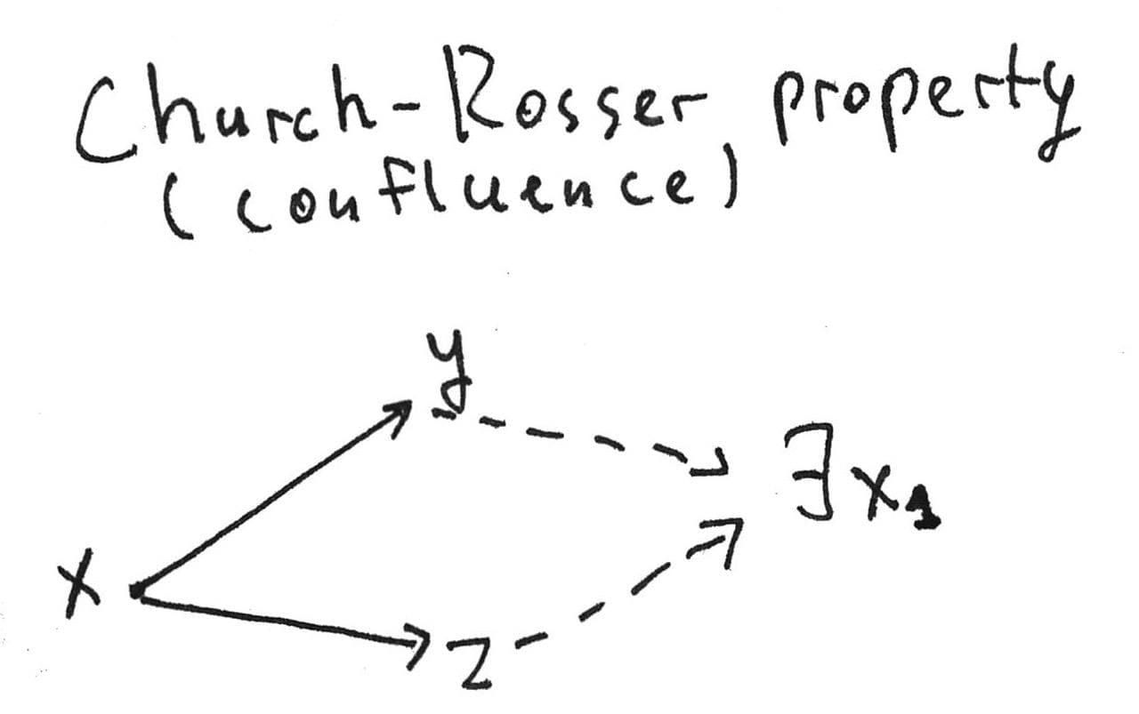
Also we may make this table that describes the correspondence between modal formulas:
| Name | Modal formula | Relation |
|---|---|---|
| for all , | ||
| for all , and implies | ||
| Seriality: for all there exists such that | ||
| Church-Rosser property (confluence): if and , then there exists such that and | ||
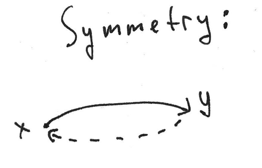
| Symmetry: for all , implies |
Let us take a look at the corresponding frame properties on a picture:
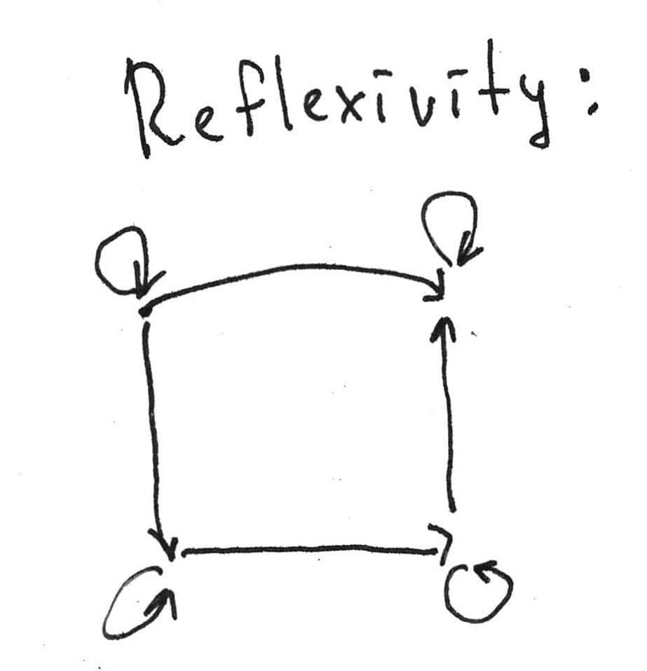
More formally and generally, a modal formula defines (or characterises) the class of frames , if for each frame ,. That is, a formula characterises the class of all reflexive frames, etc.
It is clear that our list is incomplete as this blog post itself, but we have described the most popular formulas and the corresponding relation properties. By the way, one may obtain new modal logics adding one of these formulae as axioms and get a botanic garden of modal logics. There are three columns in the following table. The first column is the name of the concrete logic, a sort of identification mark. The second column describes how the given logic is axiomatised. Generally, denotes that we extend minimal normal modal logic with formulas from as the additional axioms. The third column is the completeness theorem that claims that a given logic is the set of formulas that are valid in some class of Kripke frames.
| Name | Logic | Frames |
|---|---|---|
| The logic of all reflexive frames | ||
| The logic of all transitive frames | ||
| The logic of all serial frames | ||
| = | The logic of all preorders (reflexive and transitive relations) | |
| The logic of all confluent preorders (preorders that satisfy the Church-Rosser property) | ||
| The logic of all equivalence relations |
The fact that a given logic is the logic of some class of frames tells us that this logic is complete with respect to this class. For instance, when we tell that is the logic of all reflexive frames, it means that any formula which is valid in an arbitrary reflexive frame is provable in . One may prove the corresponding completeness theorem ensuring that the formulas from the table are canonical ones.
A modal formula is called canonical, if the logic is the logic of its canonical frame. It’s not difficult to ensure that if logic has an axiomatisation with canonical formulas, then this logic is Kripke complete. For example, if we want to prove that is the logic of all preorders, it’s enough to check that the relation on the -canonical frame is a preorder.
Let us remember first-order logic once more. The first is to rewrite the first table above changing the properties for the third column with the relevant first-order formulas as follows:
| Name | Modal formula | Property of a frame written in the first-order language |
|---|---|---|
The current question we would like to ask is there some bridge between modal formulas and first-order properties of relation in a Kripke frame. Before that, we introduce a fistful of definitions.
A modal formula is called elementary if the class of frames which this formula characterises is defined by some first-order formula. For example, the formulas from the table above are elementary since the corresponding frame properties might be arranged as well-formed first-order formulas.
Let us define the special kind of formulas that we call Sahlqvist formulas:
A box-atom is a formula of the form or , where is a finite (possibly, empty) sequence of boxes. A Sahlqvist formula is a modal formula of the form . is a -sequence of boxes, . is formula that contains , , , , perhaps, times. is constructed from box-atoms, and .
For instance, any formula from our table is a Sahlqvist formula. The example of a non-Sahlqvist formula is the McKinsey formula , which is also non-elementary. This formula should be a separate topic for an extensive discussion. The reader may continue such a discussion herself with the classical paper by Robert Goldblatt called The McKinsey Axiom is not Canonical.
Theorem (Sahlqvist’s theorem)
Let be a Sahlqvist formula, then is canonical and elementary.
Sahlqvist’s theorem is extremely non-trivial to be proved accurately in detail. However, this theorem gives us crucially significant consequences. If some normal modal logic is defined with Sahlqvist formulas as axioms, then it’s automatically Kripke complete since every axiom is canonical and elementary.
Moreover, any Sahlqvist formula defines some property of a Kripke frame which is definable in the first-order language. The modal definability of first-order properties in itself has certain advantages. Let us observed them concisely and slightly philosophically. As we said at the beginning, a modal language extends the propositional one with unary operators and . As the reader could have seen, necessity and possibility have connections with universality and existence. We established this connection defining the standard translation and embedding the minimal normal modal logic into the first-order predicate logic.
On the one hand, it is a well-known result that first-order logic is undecidable. Thus, we don’t have a general procedure that defines whether a given first-order formula is true or not (alternatively, provable or not). On the other hand, we have already observed the analogy between quantifiers and modalities. On the third hand (yes, I have three hands, it’s practically useful sometimes), modal logics are mostly decidable as we will see a little bit later.
That is, one has a method to check the validity of some binary relation properties by encoding them in modal logic. Such a way doesn’t work for an arbitrary property, indeed. But a large class of such characteristics might be covered via modal language. In the second part, we also take a look at the example of a formula whose class of Kripke frames is not first-order definable.
In order to remain intellectually honest, we should note quite frankly and openly that there also exist first-order properties of Kripke frames which are undefinable in a modal language. A relation is called irreflexive, if it is false that for each . The example of an irreflexive relation is the set of natural numbers with , just because there is no natural number that could be less than itself, indeed.
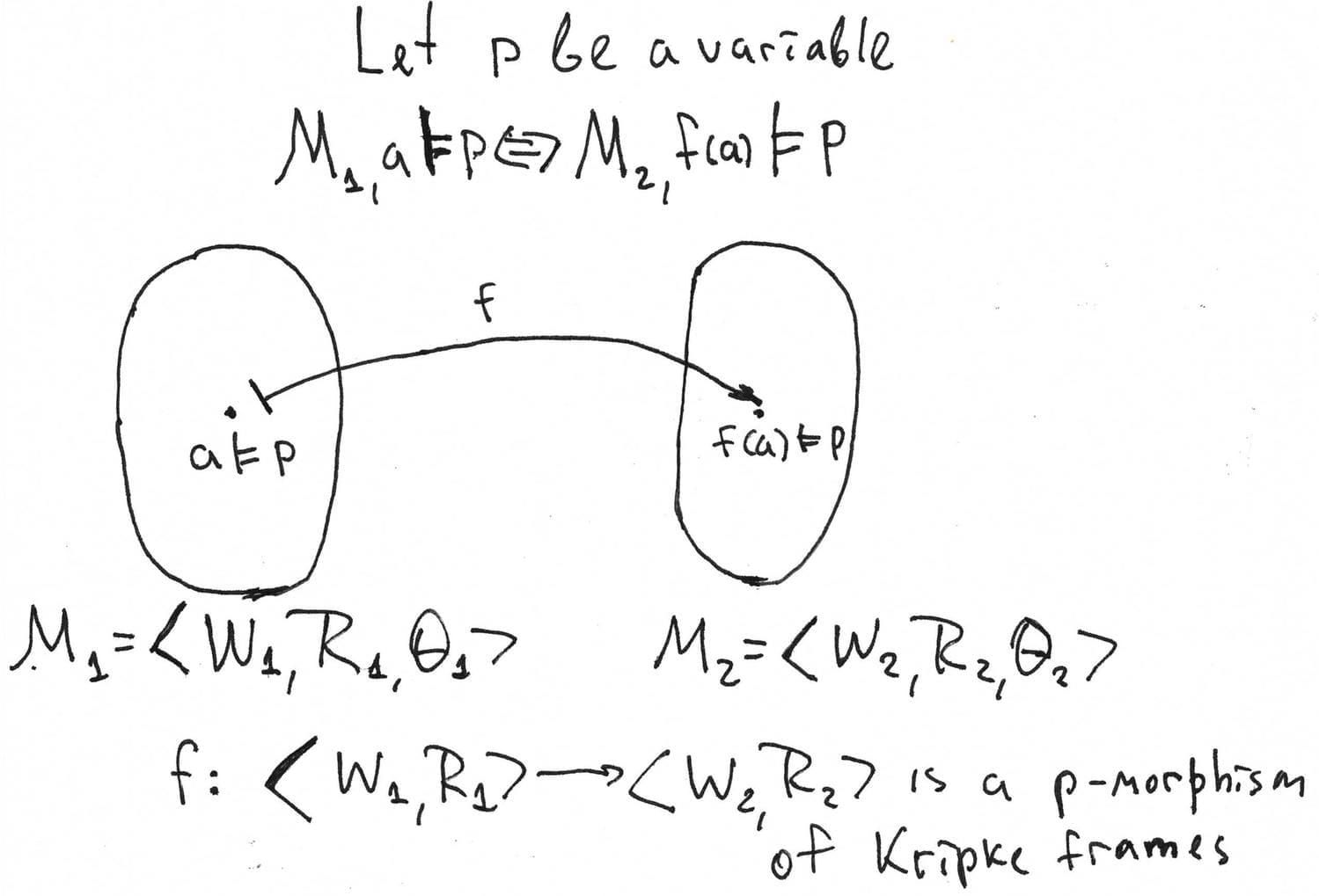
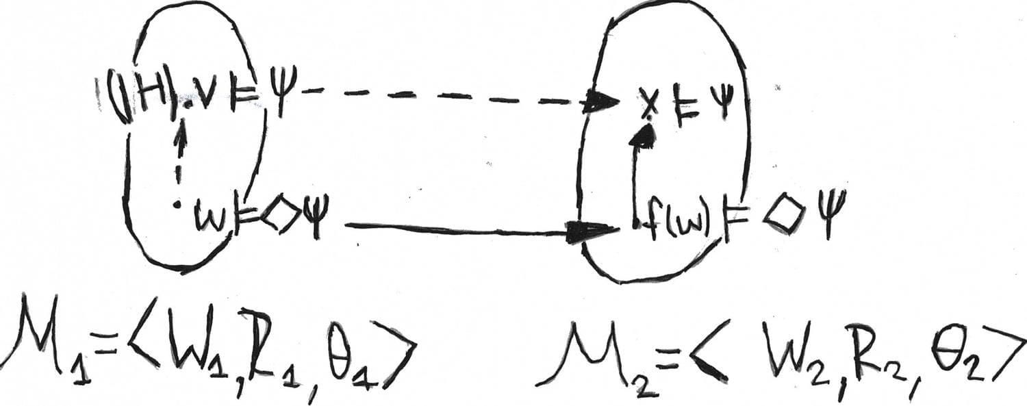
Let us define the notion of -morphism, a natural homomorphism between Kripke frames. By natural homomorphism, we mean a map that preserves a structure of Kripke frame and validness at the same time. Let us explain the idea with the precise definition and related lemma.
Definition
Let , be Kripke frames, then -morphism is a map such that:
- is monotone, i. e., implies :
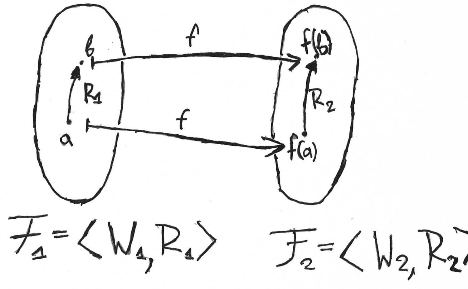
- has a lifting property, i. e., implies that there exists and

A -mophism between Kripke models , is a -morphism such that:
for every variable .
If is a surjective -morphism, then we will write . By surjection, we mean a map such that for each there exists such that .
The following lemma describes a -morphism behaviour with formulas that are true in models and valid in frames.
Lemma
- If , then iff
- If , then
Proof
We prove only the first part of the lemma. Let us suppose that is a primitive modality for a technical simplicity. The base case with variables is already proved since the condition of the lemma for variables is the part of model -morphism definition.
Let us assume that . We prove that iff . In other words, one needs to prove two implications:
- If , then .
Let , then there exists such that . By induction hypothesis, . is a -morphism, hence is monotone and implies . Thus, . We visualise the reasoning above as follows:
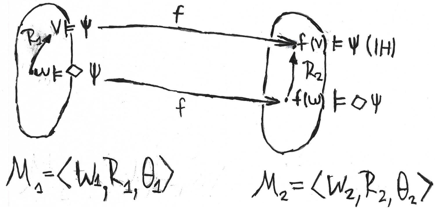
- If , then
Let . Then there exists such that . is a -morphism and , then there exists such that and . By induction hypothesis, . But , so . Take a look at the picture.
Now we show that there doesn’t exist a modal formula that expresses irreflexivity of a relation.
Lemma The class of all irreflexive frame is not modal definable.
Proof Let be a Kripke frame, a natural numbers with less-than relation, which is obviously irreflexive. Let . Let us put as for all .
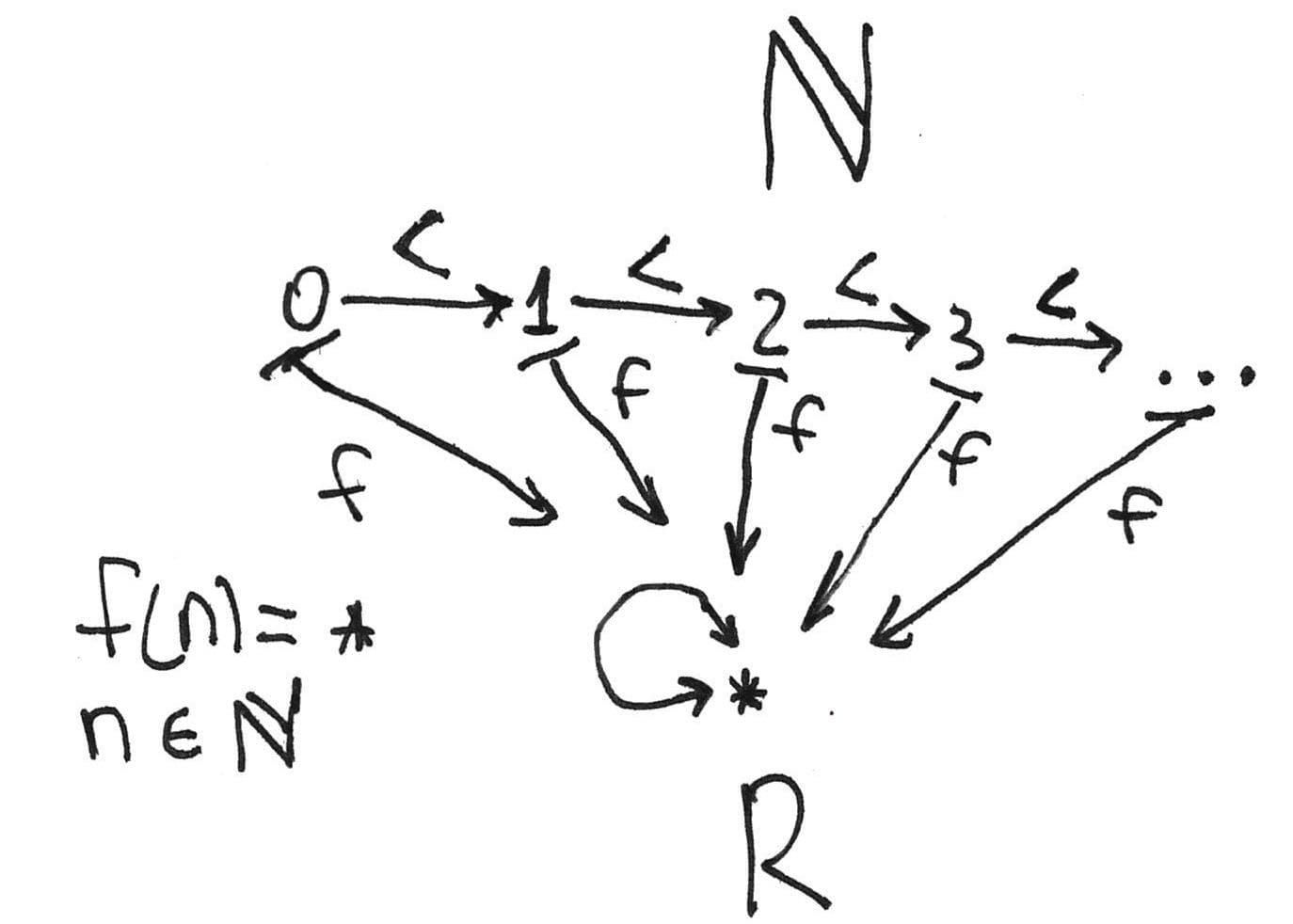
It is easy to see that this map is monotone and surjective. Let us check the lifting property. Let . Let , then and . Then is a -morphism, but is an irreflexive frame and is merely reflexive point.
If the reader is interested in modal definability in more detail, then she might take into consideration the Goldblatt-Thomason theorem that connects modal definability, first-order definability with -morphisms and some other operations on Kripke frames for further study.
Decidability in modal logic
The decidability of a formal system allows one to establish whether a formula is provable or not algorithmically. In modal logic, the famous Harrop’s theorem provides the most widespread method of decidability proving. Let us introduce some definitions to formulate this theorem.
Definition
A normal modal logic is finitely axiomatisable if for some , where is a finite set of formulae.
In other words, is finitely axiomatisable if this logic extends minimal normal modal logic with some finite set of axioms.
Definition
A normal modal logic has a finite model property (or finitely approximable), if , where is some class of finite frames.
That is, a finite model property is a Kripke completeness with respect to the class of finite Kripke frames. Now we formulate the famous Harrop’s theorem:
Theorem (Harrop)
Let be a normal modal logic such that is finitely axiomatisable and has a finite model property. Then is decidable.
Proof
We provide only a quite brief proof sketch. It is clear that the set of formulas provable in is enumerable since this logic merely extends with the finite set of axioms. On the other hand, let . Then the set is also enumerable, so far as one may enumerate finite frames such that and , where .
So, if we have some finitely axiomatisable logic, then one needs to can show that this logic is complete with respect to some class of finite frames. Here, we will assume that is a primitive modality for simplicity.
Definition
Let be a Kripke model and a set of formulas closed under subformulas (that is, if and is a subformula of , then ). We put the following equivalence relation:
, where
Then, a filtration of a model through a set is a model , where
- . In other words, is a quotient by relation , the set of equivalence classes.
- Let , then
Here is a quite obvious observation. Suppose, one have a model and its filtration through the set of subformulas , where is a arbitrary formula. Then .
Harrop’s theorem provides the uniform method to prove that some normal modal logic is decidable if this logic is finitely axiomatisable and has finite model property. We need filtration to prove that a given logic is finitely approximable.
Here comes the first lemma about minimal filtration.
Lemma
Let be a Kripke model and a set of formulas closed under subformulas, then , where .
Proof
Quite simple induction on . Let us check this statement for .
At first, let us check the only if part. Let . Then there exists such that . By induction hypothesis, . But by the definition of . This, .
The converse implication has the same level of completexity. Let . Then there exists such that . Consequently, there exist and such that . By assumption, . Thus, .
Now we may formulate the theorem which claims that the minimal normal modal logic is the logic of all finite Kripke frames.
Theorem
- , where is the class of all finite Kripke frames.
- , where is the class of all finite reflexive frames.
- , where is the class of all finite serial frames.
- , where is the class of all finite symmetric frames.
Proof
Let . It means that there exists a model and such that according to the completeness theorem. Let be a minimal filtration of a model through , the set of subformulas of . By the previous lemma, . It is clear that this model is finite, since , as we observed above.
(2), (3), (4) are proved similarly, but one needs to check that a minimal filtration preserves reflexivity, seriality, and symmetry.
However, we are in trouble. We haven’t already discussed a finite model property of logics that contain transitivity as an axiom. Unfortunately, a minimal filtration doesn’t have to preserve the transitivity. Let be a transitive model and a minimal filtration of through . Let such that and . If , then there exists and such that . From the other hand, if , then there exists and such that .
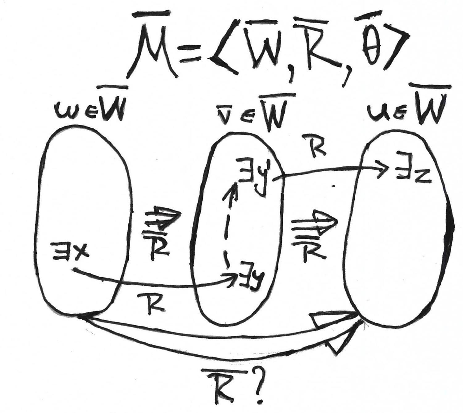
It is clear that doesn’t have to see within the equivalence class . Thus, a relation in minimally filtrated model isn’t necessarily transitive, even if the original relation is transitive.
A solution to that problem is the transitive closure of a relation in a minimal filtration. Let us discuss what a transitive closure is. Suppose we have some set with a binary relation . Generally, this relation is not transitive, but we’d like to extend it to the transitive one. What should we make? Suppose we have such that and . We add to the extended relation which we denote as . We perform this action for each situation. That gives us a transitive version of a relation.
Here we going to extend a relation in a minimal filtration. This solution was proposed initially by Dov Gabbay. We will denote this closure .
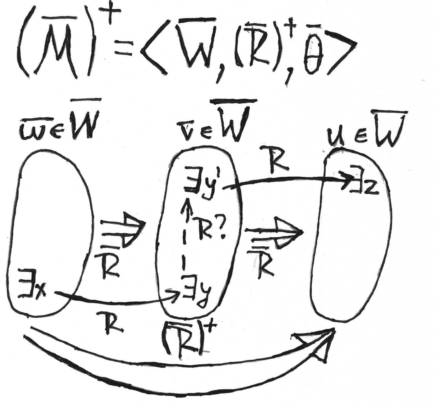
A transitive closure of a relation in a minimal filtration allows us to prove that is the logic of finite transitive frames. Firstly, we formulate the lemma that explains why a transitive closure is a good idea:
Lemma
Let be a transitive model and a minimal filtration through , then the following conditions hold:
- If , then , where . This statement claims that a relation in a minimal filtration is a subrelation if its transitive closure.
- If , then . If two relation are connected with the underlying relation, then a transitive closure preserve this connection.
- Let and , then . Here we claim that a transitive closure should respect the truth condition for .
Using the lemma above, it is not so hard to obtain the following theorem:
Theorem
- , where is the class of all finite transitive frames
- , where is the class of all finite preorders.
- , where is the class of all finite equivalence relations.
The theorem above allows us to claim that the logics , , and have a finite model property. All these logics are finitely axiomatisable. Then, by Harrop’s theorem, , , and are decidable. That is, one has a uniform method to provide a countermodel in which every unprovable formula fails.
Summary
We discussed a brief history of modal logic and its mathematical and philosophical roots. After that, we introduced the grammar of modal logic to define what modal formula is. As we have already told, the definition of a modal language is not enough to deal with modal logic. From a syntactical perspective, we have formal proofs as derivation with axioms and inference rules. We defined normal modal logic as a set of formulas with specific limitations. As an underlying logic, we fixed minimal normal logic . Here, the other modal logics merely extend the minimal normal modal one with the additional axioms. Note that syntax doesn’t answer the question about the truth of a formula. The distinction between proof and truth is a foundation of the logical culture in itself. Truth is a semantical concept.
To define the truth condition for modal formulas, we defined Kripke frames and Kripke models. After that, we formulated the completeness theorems for the list of modal logics. As usual, completeness tells us that, very roughly speaking, any valid formula is provable. The underlying modal logic is a logic of all possible Kripke frames. Other modal logics are complete with respect to a narrower class of frames with the relation in which is restricted somehow. Alright, we have the completeness theorem for some logic, but we also would like to define whether a given formula is provable or not algorithmically. For this purpose, we took a look at methods of proving the fact that a given normal modal logic has finite model property. Finite model property with finite axiomatisation gives us decidability according to the Harrop’s theorem.
We studied the background of modal logic so that we could continue our journey in more concrete case studies. In the second part, we will overview concrete branches of modal logic, such as topological semantics, provability logic, and temporal logic. We will discuss how exactly modal logic is connected with geometry, the foundations of mathematics, and computer science.
I sincerely hope the reader managed to survive in this landscape of such an abstract and theoretically saturated material.

.jpg)
.jpg)
.jpg)