Incomplete and Utter Introduction to Modal Logic, Pt. 2

In the first part, we introduced the reader to basic modal logic. We discussed Kripke semantics, some of the popular systems of modal logic. We also observed how to prove the decidability of modal logics using such tools as minimal filtration and its transitive closure. Here we observe use cases and take a look at connections of modal logic with topology, foundations of mathematics, and computer science. Finally, we recommend the literature for further reading and study.

Brief introduction to topology and metric spaces

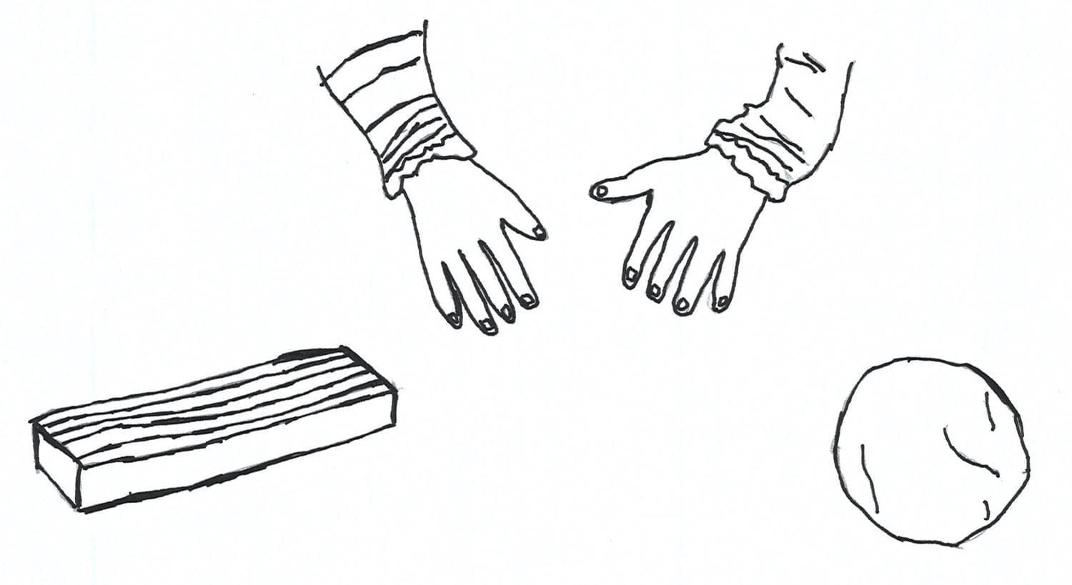
Topology is the branch of mathematics that studies geometric objects such as planes, surfaces, and their continuous deformations. The notion of a continuous deformation might be illustrated with an example. Suppose you have a cube-shaped piece of plasticine. You deform that piece into the sphere continuously, i. e., keeping your hands on that piece all the time:

Topology study geometric structures up to homeomorphism. A homeomorphism is a one-to-one continuous transformation as in the example above.

The abstract definition of a topological space is set-theoretical. A topological space is defined as a family of subsets. More formally, a topological space is a pair $\mathcal{X} = \langle X, \tau \rangle$, where $X$ is a non-empty set and $\tau$ is a family of subsets of $X$ with the following data:

1. $\emptyset, X \in \tau$
2. If $A, B \in \tau$, then $A \cap B \in \tau$
3. Let $I$ be an indexing set and for each $i \in I$ $A_i \in \tau$, then $\bigcup \limits_{i \in I} A_i$. Here, an indexing set is an arbitrary set that might have any cardinality. If $A \subseteq X$ and $A \in \tau$, then we call $A$ an open set. A subset $A \subseteq X$ is called closed, if $A$ is a complement of some open set.

The most common practice is defining a topological structure via a base of topology. A base of topology is a family of opens such that every open set in this space has the form of union of some elements from the base. We consider instances of a base within examples of topological spaces.

Examples of topological spaces are:

1. Let $X$ be a set and $\mathcal{P}(X)$ a set of all subsets of $X$, then $\langle X, \mathcal{P}(X) \rangle$ is a topological space, in which every subset is open. We call such a space discrete since its base is the set of all singletons $\{x\}$, $x \in X$.
2. Let $X$ be a set and $\tau = \{ \emptyset, X \}$, then $\langle X, \tau \rangle$ is also space, where only the underlying set and the empty one are open. $\langle X, \tau \rangle$ is called anti-discrete space.

The topologies above are trivial ones. Let us consider a slightly more curious example.

Let $\langle X, \rho \rangle$ be a metric space. By metric space, we mean a set equipped with a distance function $\rho : X \times X \to \mathbb{R}_{\geq 0}$ that every pair of points maps to some non-negative real number, a distance between them. A distance function has the following conditions:

1. $\rho(x, x) = 0$. The distance between the point with itself equals to zero.
2. $\rho(x, y) = \rho(y, x)$. The distance between points doesn’t depens on the arguments order.
3. $\rho(x, z) \leq \rho(x, y) + \rho(y, z)$. The triangle inequation.

One may topologise any metric space uniformly. Let $\varepsilon$ be a positive real number and $x \in X$. An open ball of radius $\varepsilon$ and centre $x$ is the set $U_{\varepsilon}^x = \{ y \in X \: | \: \rho(x, y) < \varepsilon \}$.

To visualise the notion of an open ball, just imagine you take a cricket ball. An open ball derived from a given cricket ball is just the content, if we assume that its content is restricted by its leather cover. The centre of a cricket ball is a centre in the usual Euclidean sense. The radius of such an open ball approximately equals to 3.5 centimetres according to International Cricket Council data.

The set of all open balls in this metric space forms the base of topology. Thus, any metric space is a topological one. Moreover, topological spaces historically arose as the generalisation of metric spaces at the beginning of the previous century.

The example of a metric space is real numbers with the distance function defined with the absolute value of subtraction. The second example is a normed vector space, a vector space equipped with a norm function, a generalisation of a vector length. One may produce a metric space from a normed vector one by defining the distance between two vectors as the norm of their subtraction. Such a metric is often called the Minkowski distance. We don’t consider the examples above in detail since those topics are closer to functional analysis and point-set topology rather than modal logic.

Closure and interior operators

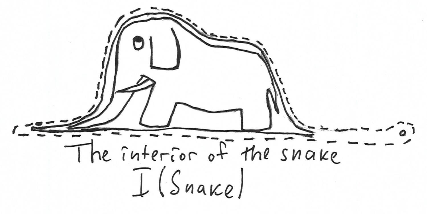
Let us motivate interior and closure as follows. Suppose we have a snake on the Euclidian plane $\mathbb{R}^2$. Unfortunately, this snake ate an elephant and lost its full-contour line after that:

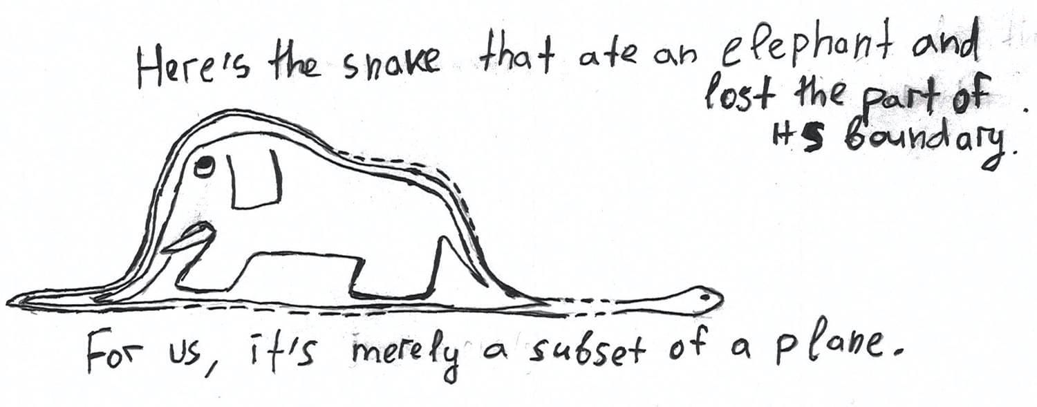
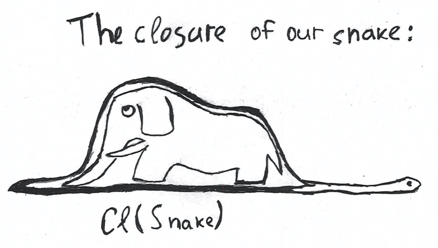
A closure operator on the Euclidean plane helps it to restore the lost part of a boundary:

We would like to identify the other regions of this snake. An interior of the snake is its container. The last sentence is not meant to be taken literally in the anatomical sense:

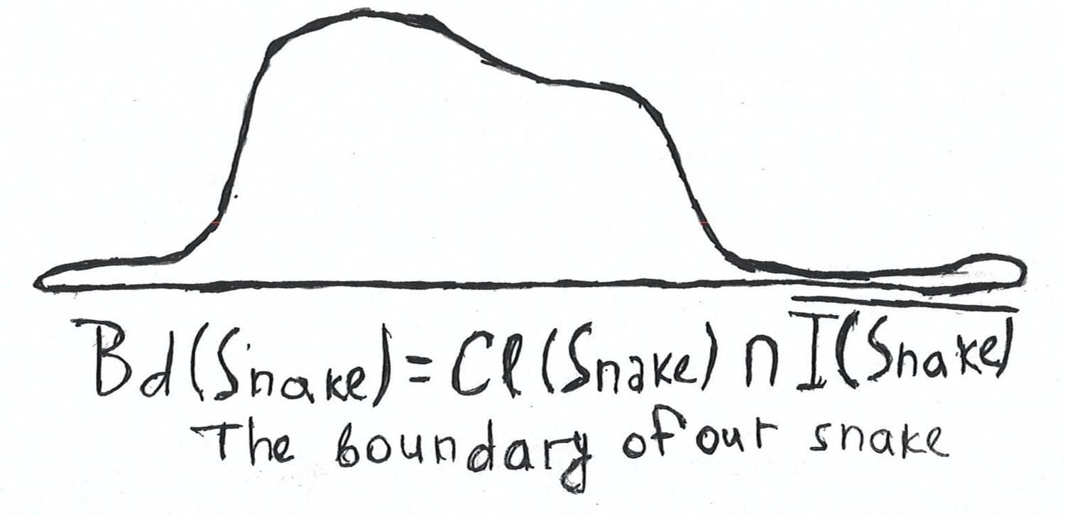
The boundary of a snake is its full contour-line without the interior. Here we are not interested in the rich inner world of our snake, only in its external borders. Just imagine that you chalked the snake:

The exterior of a snake is the whole plane without this snake itself. An exterior operator allows the snake to define strictly what an external world is:

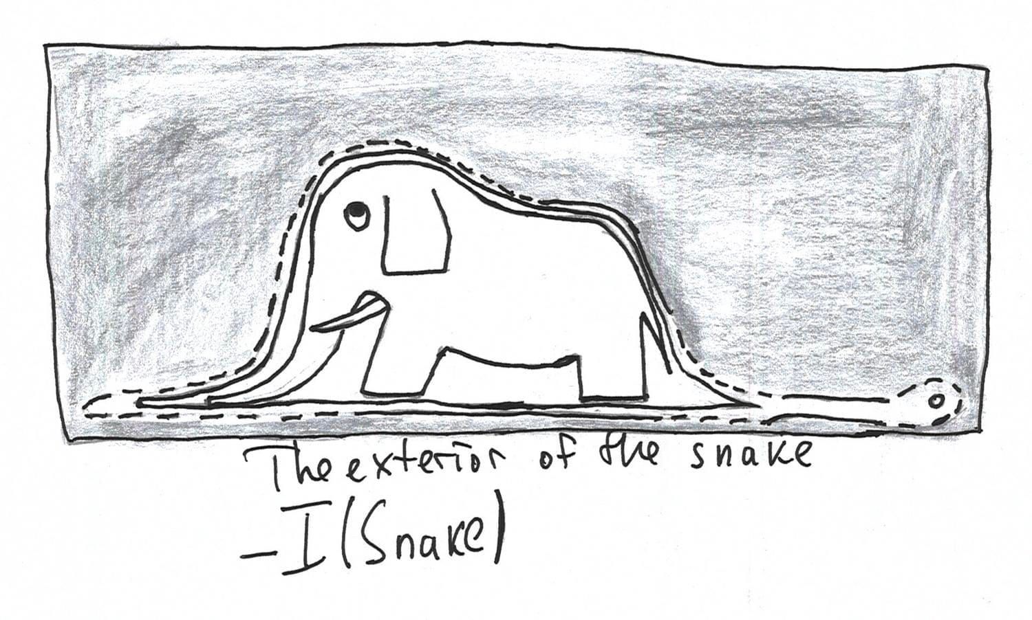
Here, the snake is the subset of plane $\mathbb{R}^2$, namely, $S$. Let us denote its closure as $\operatorname{Cl}S$. $\operatorname{I}S$ is its interior. The boundary of a snake is the closure of the snake minus its interior, $\operatorname{Cl} S \cap - \operatorname{I} S$. The exterior of this snake is an interior of its complement. Here the basic notions are interior and closure. Let us move on to stricter definitions:

Let $\mathcal{X} = \langle X, \tau \rangle$ be a topological space and $A \subseteq X$ a subset of $\mathcal{X}$. A closure of $X$ is the smallest closed set that contains $X$. More precisely:

$\operatorname{Cl}(X) = \bigcap \{ A \in \operatorname{Closed}(\mathcal{X}) \: | \: X \subseteq A \}$

A closure operator satisfies the following properties that also knows as Kuratowski’s axioms:

$\operatorname{Cl}(\emptyset) = \emptyset$, empty set is closed. $A \subseteq \operatorname{Cl}A$, any set is a subset of its closure. $\operatorname{Cl}A = \operatorname{Cl}\operatorname{Cl}A$, you don’t need to apply closure operator twice, it’s idempotent. $\operatorname{Cl}(A \cup B) = \operatorname{Cl}A \cup \operatorname{Cl}B$, a closure operator distributres over finite union.

Very and very roughly speaking, a closure operator transforms any subset to a closed one. A dual operator is an interior. An interior of a subset $X$ is the biggest open subset of $X$: $\operatorname{I}(X) = \bigcup \{ A \in \tau \: | \: A \subseteq X \}$.

It is not so hard to show that $\operatorname{I}(X) = - (\operatorname{Cl}(- X))$ since an open set is a complement of a closed one and vice versa. An interior operator satisfies the following conditions: $\operatorname{I}X = X$ $\operatorname{I}A \subseteq A$ $\operatorname{I}A = \operatorname{I}\operatorname{I}A$ $\operatorname{I}(A \cap B) = \operatorname{I}A \cap \operatorname{I}B$

To observe the analogy between Kuratowski’s closure axioms and the logic ${\bf S}4$, let us take a look at the equivalent formulation of ${\bf S}4$. We recall that ${\bf S}4$ is a normal modal logic that extends ${\bf K}$ with reflexivity and transitivity axioms:

1. Boolean tautologies
2. The Kripke axiom $\Box (p \to q) \to (\Box p \to \Box q)$
3. $\Box p \to p$
4. $\Box p \to \Box \Box p$ Inference rules: Modus Ponens, Substitution, Necessitation.

First of all, we define a normal modal logic as the set of formulas that consists of all Boolean tautologies, the following two formulas:

1. $\Diamond p \lor \Diamond q \leftrightarrow \Diamond (p \lor q)$
2. $\Diamond \bot \leftrightarrow \bot$ and closed under Modus Ponens, Substitution, and monotonicity rule: from $\varphi \to \psi$ infer $\Diamond \varphi \to \Diamond \psi$.

The reader might check that this definition of normal modal logic is equivalent to the definition we introduced in the first part as an exercise.

The minimal normal modal logic is the least set of formulas that satisfy the previous conditions. Such a logic is deductively equivalent to ${\bf K}$ defined in the previous post. Then ${\bf S4}$ is an extension of the minimal normal modal logic with reflexivity and transitivity axioms, more explicitly:

1. $\Diamond p \lor \Diamond q \leftrightarrow \Diamond (p \lor q)$
2. $\Diamond \bot \leftrightarrow \bot$
3. $p \to \Diamond p$
4. $\Diamond \Diamond p \to \Diamond p$

As the reader could see, the ${\bf S4}$ axioms are the same as the Kuratowski’s closure axioms if we read $\operatorname{Cl}$ as $\Diamond$. Dually, we represent ${\bf S}4$ logic with boxes and observe the analogy with the Kuratowski’s interior axioms, if we read $\operatorname{I}$ as $\Box$:

1. $\Box p \land \Box q \leftrightarrow \Box (p \land q)$
2. $\Box \top \leftrightarrow \top$
3. $\Box p \to p$
4. $\Box p \to \Box \Box p$

We may study such an analogy considering topological models (or topo-models) in which we define the truth condition for modalities via open and closed sets in a given topological space.

Topological models

We discussed Kripke-style semantics based on binary relations before. The idea of topological models is the same, but we replace Kripke frames with topological spaces and modal formulas are understood in terms of closed and open sets.

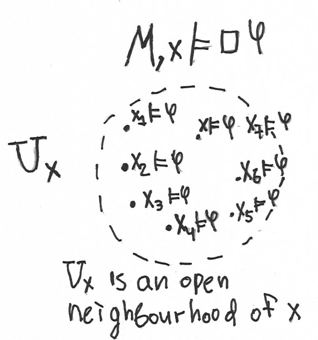
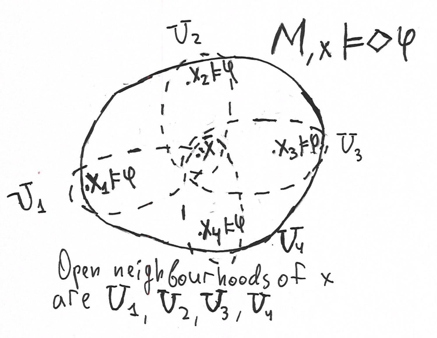
Let $\mathcal{X} = \langle X, \tau \rangle$ be a topological space and $\vartheta : \operatorname{PV} \to 2^{X}$ be a valuation. A topological model is a triple $\mathcal{M} = \langle \mathcal{X}, \vartheta \rangle$ with the following thurh conditions. Here we assume that $\neg$, $\lor$, and $\Box$ are primitive connectives:

1. $\mathcal{M}, x \models p \Leftrightarrow x \in \vartheta ( p )$
2. $\mathcal{M}, x \models \neg \varphi \Leftrightarrow \mathcal{M}, x \nvDash \varphi$
3. $\mathcal{M}, x \models \varphi \lor \psi \Leftrightarrow \mathcal{M}, x \models \varphi \text{ or } \mathcal{X}, x \models \psi$
4. $\mathcal{M}, x \models \Box \varphi \Leftrightarrow$ there exists an open neighbourhood $U$ such that $x \in U$ and for each $y \in U$ $\mathcal{M}, y \models \varphi$

Let us define that valuation of an abritrary formula that follows from the semantics above:

1. $||p|| = \vartheta(p)$
2. $||\neg \varphi|| = - ||\varphi||$
3. $||\varphi \lor \psi|| = ||\varphi|| \lor ||\psi||$
4. $||\Box \varphi|| = \operatorname{I}(||\varphi||)$, that is, $\Box$ is exaclty an interior in terms of topological semantics.

As in Kripke models, a valuation function maps each variable to some subset of an underlying set. From a naive geometric intuition, a valuation function determines some region on a space. If we return to our example with the snake on a plane, then we may, for example, require that $\vartheta ( p ) = S$. The items 2-3 are the same as in Kripke models. The truth condition for $\Box$ is completely different. Logically, this condition declares that $\Box \varphi$ is true at the point $x$ if $\varphi$ is locally true. It means that the proposition $\varphi$ is true at each point in some region of an observed space.

As we remember, $\Diamond = \neg \Box \neg$. Thus, the possibility modality has the following truth condition in a topological model:

$\mathcal{M}, x \models \Diamond \varphi \Leftrightarrow$ for each open neighbourhood $U$ such that $x \in U$ there exists $y \in U$ such that $\mathcal{M}, y \models \varphi$. In other words, there exists a point in every open neighbourhood $U$ of $x$ at which $\varphi$ is true. This definition induces the closure of $||\varphi||$, the set of all points at which $\varphi$ is true: $||\Diamond \varphi|| = ||\neg \Box \neg || - (\operatorname{I} (- ||\varphi||)) = \operatorname{Cl}(||\varphi||)$

Also, we will use the same notation as in Kripke semantics: $\mathcal{M} \models \varphi$ iff $\varphi$ is true at every point. $\varphi$ is valid in a topological space iff it’s true in every model on this space. The logic of a topological space $\mathcal{X}$ is the set of valid formulas in this space. The logic of class of topological space is an intersection of logics.

In Kripke semantics, the logic ${\bf K}$ was the underlying one, ${\bf K}$ is the logic of all Kripke frames. The same question for topological spaces is quite natural. McKinsey-Tarski theorem claims that ${\bf S}4$, the logic of all preorders from a Kripkean perspective, is the logic of all topological spaces. Let us discuss the soundness theorem first. Moreover, any extension of ${\bf S}4$ is complete with respect to some class of topological spaces.

Theorem Let $\mathbb{X}$ be a class of all topological spaces, then ${\bf S}4 = \operatorname{Log}(\mathbb{X})$

Proof Let us prove that ${\bf A}4 = \Box p \to \Box \Box p$ is valid. Let $\mathcal{X}$ be a topological space and $\vartheta$ a valuation. Let $\mathcal{M}, x \models \Box p$. Then there exists an open neighbourhood $U_x$ such that for each $y \in U_x$ $\mathcal{M}, y \models p$. $y \in U_x$, then $U_x$ is also open neighbourhood of $y$. Thus, $\mathcal{M}, y \models \Box p$ and $\mathcal{M}, x \models \Box \Box p$.

To prove the converse inclusion, one needs to perform the same thing as in the case of Kripke semantics. The set of all maximal ${\bf S}4$-consistent sets forms a topological space. So, one can build a canonical topological model, a topo-model on the set of all maximal ${\bf S}4$-consistent sets with canonical valuation. We refer the reader to the paper called Reasoning About Space: The Modal Way written by Marco Aiello, Johan van Benthem, and Guram Bezhanishvili, where the topological completeness of ${\bf S}4$ is shown quite accurately. Thus, ${\bf S}4$ is the logic of all topological spaces.

Some might say that this is result is too abstract. We would like to take a look at a more precise classification of topological spaces with modal logic. Modal logic is able to provide an invariant for topological spaces, but, frankly speaking, it’s quite weak. Let us observe, however, what had already been done in topological semantics of modal logic. In other words, we discuss how we can particularise the class of topological spaces preserving McKinsey-Tarski theorem.

Let $\mathcal{X}$ be a discrete space, then $\operatorname{Log}(\mathcal{X}) = {\bf K} \oplus \Box p \leftrightarrow p$. This axiom claims that we may box and unbox everywhere. From a topological point of view, it denotes that the interior operator is the trivial one. That is, any subset is open. All modalities fade away since the interior operator is merely the identity function on subsets.

Let $\mathcal{X} = \langle X, \tau \rangle$ be an infinite anti-discrete space, that is, only $X$ and $\emptyset$ are open, then ${\bf S}5 = \operatorname{Log}(\mathcal{X})$. As we told in the first part, ${\bf S}5 = {\bf S}4 \oplus p \to \Diamond \Box p$. The last axiom expresses symmetry of a relation. The symmetry formula also has the equivalent form $\Diamond \Box p \to p$.

The truth condition for $\Box$ in models on anti-discrete spaces transforms as follows. $\Box \varphi$ is true at the point $x$, if there exists an open neighbourhood $U_x$ such that $\mathcal{M}, y \models \varphi$. In an anti-discrete space, there is only the one open neighbourhood for every point, the space itself. That is, in an anti-discrete space, $\mathcal{M}, x \models \Box \varphi$ iff $\mathcal{M}, y \models \varphi$ for each $y \in X$. It’s not hard to check that ${\bf AB}$-axiom is valid on every infinite anti-discrete space. Let $x \in X$ and $\mathcal{M}, x \models \Diamond \Box \varphi$. Then for every open neighbourhood $U_x$ there exists the point $y$ such that $\mathcal{M}, y \models \Box \varphi$. But there is only one open neighbourhood of $x$, the space itself. Thus, $\mathcal{M}, x \models \varphi$.

Let $\mathcal{F} = \langle W, R \rangle$ be a preorder, that is, ${\bf S}4$-frame. One may induce a topological structure on a preorder if we take also upper sets as opens. A set $A \subseteq W$ is called upper if $x \in A$ and $x R y$ implies $y \in A$. In this topology, any intersection of opens is open, or equivalently, the interior operator distributes over an arbitrary intersection of subsets. Such a space is the instance of Alexandrov space. This connection claims that topological semantics for modal logic generalises Kripkean semantics for ${\bf S}4$ and its extensions.

${\bf S}4$ is also the logic of the class of all metric spaces as it was proved by McKinsey and Tarski. Rasiowa and Sikorski showed that ${\bf S}4$ is the logic of all dense-in-itself metric spaces, that is, metric spaces that contain no isolated points. Here we may claim that modal logic provides invariants for topological and metric spaces, but such invariants are too rough if we have closure and interior modalities. The roughness of these invariants follows from the fact that all topological spaces, all metric spaces and all dense-in-itself metric spaces have exactly the same logic and those spaces are indistinguishable from a logical point of view.

We refer the reader to the paper by Guram Bezhanishvili, David Gabelaia, and Joel Lucero-Bryan to become familiar with more precise classification of modal logics of metric spaces.

Note that interior and closure are not the only topological modalities. There are also a so-called graduated, tangled, difference, and other modal operators that are of interest from a topological perspective. Such extensions of modal language allow one to study topological and metric spaces from a logical perspective much more faithfully. You may read the recent paper by Ian Hodkinson and Robert Goldblatt called Strong completeness of modal logics over $0$-dimensional metric spaces, where those alternative modalities are overviewed quite clearly. Also, you may read the paper Some Results on Modal Axiomatisation and Definability for Topological Spaces by Guram Bezhanishvili, Leo Esakia, and David Gabelaia to understand the expressive power of so-called derivation modality that generalises closure in some sense. Let us observe briefly a universal modality as an example of such an additional modality.

The universal modality is denoted as $[\forall]$ and has the following semantics: $\mathcal{M}, x \models [\forall] \varphi \Leftrightarrow$ $\mathcal{M}, y \models \varphi$ for each $y \in \mathcal{X}$, where $\mathcal{X}$ is an underlying topological space.

The modal logic that we seek is the system ${\bf S}4{\bf U}$ which is defined in the bimodal language. We have $\Box$ (an interior modality) that satisfies ${\bf S}4$ axioms and we have $[\forall]$ with ${\bf S}5$ axioms. We also add the additional postulate that has the form $[\forall] p \to \Box p$. That is, if the statement is true everywhere, then it’s true in every open neighbourhood. The very first example of a universal modality is an interior operator in an infinite anti-discrete space, as we observed above. In other words, universal modality is stronger than the interior. Logically, $[\forall] \varphi$ denotes that $\varphi$ is true at every point. A formula $\Box \varphi$ tells us that $\varphi$ is locally true, i. e. at some open neighbourhood that shouldn’t cover the whole space. Moreover, there is the result according to which ${\bf S}4{\bf U}$ is the logic of arbitrary zero-dimensional spaces, such as Cantor space, or rational numbers as a metric space with the usual distance.

Also we observe the following postulate:

$[\forall](\Box p \land \Box \neg p) \to [\forall] p \vee [\forall] \neg p$

This formula denotes the fact that an observed space is connected one, i.e. we cannot split it into two disjoint open subsets. Informally, formula claims that if one can split whole space into two disjoint subsets, then one of them is empty. More formally. Let $\mathcal{X}$ be a topological space, then $\mathcal{X} \models [\forall](\Box p \land \Box \neg p) \to [\forall] p \vee [\forall] \neg p$ if and only is $\mathcal{X}$ is connected. Moreover, ${\bf S}4{\bf U} \oplus [\forall](\Box p \land \Box \neg p) \to [\forall] p \vee [\forall] \neg p$ is the logic of all connected separable dense-in-itself metric spaces.

Modal logic and provability. Modal logic meets foundations of mathematics

As we noticed previously, one may study provability and consistency in arithmetic via modal logic. The problem of provability and consistency in Peano arithmetic (briefly, ${\bf PA}$) is connected with famous Gödel’s incompleteness theorems. To understand the connection between modal logic and these aspects of ${\bf PA}$, we show how to prove the incompleteness theorems. Before that, let us explain the historical context of the Gödel’s theorems’ appearance.

At the beginning of the 20th century, one of the commonly discussed topics was the question about the foundations of mathematics and its consistency. Such mathematicians as Richard Dedekind and Georg Cantor were interested in axiomatisation of real analysis in order to describe the principles of real numbers as the set of primitive properties of the real line in terms of order and arithmetical operations.

The notion of a number was defined intuitively before, but one may define a number formally with the set theory proposed by Cantor. Unfortunately, the initial version of the set theory was inconsistent. Inconsistency of Cantor’s set theory was shown by Bertrand Russell who invited the famous paradox which is named after him. The paradox-free version of the set theory is so-called Zermelo-Fraenkel theory which is assumed sometimes as the “default” foundations of mathematics.

Later, in the 1920-s, David Hilbert, a German mathematician who famous for his works in the foundations of geometry, algebra, and mathematical physics announced the programme of establishing mathematics consistency.

According to Hilbert’s programme, any mathematical theory such as differential equations should be embedded in some formal axiomatic theory. Moreover, any usual mathematical proof must correspond to some formal proof. By formal proof, we mean a finite text written according to a set of strictly defined rules such as inference rules in first-order logic. The finite methods themselves should be formalised in Peano arithmetic, a formal axiomatic theory of natural numbers. Although, there was the open question: how can we prove that formal arithmetic is consistent within itself? In other words, we would like to formalise formal methods in Peano arithmetics and we want to have a finite proof of Peano arithmetic at the same time. Since this hypothetical proof should be finite, then it also should be formalised in Peano arithmetic.

Kurt Gödel solved this problem negatively in 1931.

More precisely, he showed that there is a sentence in Peano arithmetic that is unprovable and true at the same time. In other words, such a statement has no formal proof but it is true as a fact about natural numbers. Let us describe the idea informally. Moreover, the finite proof of ${\bf PA}$ consistency is impossible since the formula that expresses desired consistency isn’t provable.

I believe, everybody heard about the Liar paradox. Let me remind it. Suppose we have a character that always lies, for instance, Tartuffe from the same-titled comedy by Molière. Let us assume that Tartuffe claims with courage, clarity, and frankness that he’s lying.

Here we are in an embarrassing situation. If Tartuffe tells that he’s lying, hence, he lies that he’s lying. Thus, he’s telling the truth. On the other hand, he always lies by definition. Such confusion is often called the Liar paradox.

Gödel used approximately the same idea and we describe how exactly in the further proof sketch. Before that, we define Peano arithmetic as a formal theory.

Peano arithmetic

Peano arithmetic is an axiomatic theory of natural numbers with addition and multiplication. Philosophically, Peano arithmetic describe the basic properties of natural numbers with primitive operations. Formally, we put the arithmetical language, the set of primitive symbols:

1. $0$ is a constant that denotes the number which is also famous as zero.
2. $\operatorname{S}$ is a unary function symbol, an increment. C++ engineer may read $\operatorname{S}( x )$ as x++
3. $+$, $\cdot$ are binary function symbols which we read as plus and product.
4. $=$ is a binary relation symbol that denotes equality.

It is not so difficult to see that all those signs are read in accordance with our everyday intuition. To define the grammar of arithmetical formulas, we should restrict the definition of the first-order formula to the observed arithmetical language.

As in first-order logic, we have a countably infinite set of individual variables. Let us define a term first:

1. Any individual variable is a term
2. $0$ is a term
3. If $t$ is a term, then $\operatorname{S}( t )$ is a term
4. If $t_1, t_2$ are terms, then $t_1 + t_2$ and $t_1 \cdot t_2$ are terms

Informally, terms are finite strings that we read as arithmetical objects. The definition of a formula is the same as in the first-order case with the additional condition: if $t_1, t_2$ are terms, then $t_1 = t_2$ is a formula.

Now we are able to define Peano arithmetic. Here we introduce two group of axioms. Let us overview the equality axioms which completely agree with our intution:

1. $\forall x \: (x = x)$. Reflexiity of equality: every object equals to itself.
2. $\forall x \: \forall y \: (x = y \rightarrow y = x)$. Symmetry of equality.
3. $\forall x \: \forall y \: ((x = y \land y = z) \rightarrow x = z)$. Transitivity of equality.

Equality respects unary and binary operations: 5. $\forall x_1 \: \forall x_2 \: \forall y_1 \: \forall y_2 \: ((x_1 = y_1 \land x_2 = y_2) \rightarrow x_1 + y_1 = x_2 + y_2)$ 6. $\forall x_1 \: \forall x_2 \: \forall y_1 \: \forall y_2 \: ((x_1 = y_1 \land x_2 = y_2) \rightarrow x_1 \cdot y_1 = x_2 \cdot y_2)$ 7. $\forall x \: \forall y \: (x = y \Rightarrow \operatorname{S} ( x ) = \operatorname{S} ( y ))$. Informally, if $x$ and $y$ are equal, then $x + 1$ and $y + 1$ are also equal.

Equality also respects other predicates: 8. $\forall x \: \forall y \: ((x = y \land P ( x )) \rightarrow P ( y ))$ This axiom claims that if objects $x$ and $y$ are equal and the property $P$ holds for $x$, then it also holds for $y$.

We also split the arithmetical group of axioms into the following subgroups. The first group form the definition of successor function $\operatorname{S}$:

1. $\neg \exists x (0 = \operatorname{S} ( x ))$
2. $\forall x \: \forall y \: (\operatorname{S} ( x ) = \operatorname{S}( y ) \rightarrow x = y)$
3. $\forall x \: (x \neq 0 \rightarrow \exists y \: (\operatorname{S}( y ) = x))$

Recursive definitions of addition and multiplication:

1. $x + 0 = x$
2. $x + \operatorname{S}( y ) = \operatorname{S}(x + y)$
3. $x \cdot 0 = 0$
4. $x \cdot \operatorname{S}( y ) = (x \cdot y) + x$

Induction schema:

1. $A ( 0 ) \land \forall x \: (A ( x ) \to A(\operatorname{S}( x ))) \to \forall x \: A( x )$ The induction schema is an axiom schema that allows you to prove arithmetical theorems inductively. Note that the induction principle is exactly the schema, here $A$ is a metavariable on arithmetical formulas. The induction schema allows us to prove theorems that depend on parameter $n$ as follows. In the formula above, a metavariable $A$ denotes a statement that contains this parameter. Suppose we have the statement $A ( n )$ that depends on the parameter $n$. To prove that this statement holds for every natural number, we first prove that this fact of $0$. This part is often called induction base. After that we assume that $A( m )$ holds for an arbitrary $m$ and we prove $A(m + 1)$, or $A(\operatorname{S} ( m ))$ in our notation. Afterwards, we conclude that $A ( n )$ is provable for each $n \in \mathbb{N}$.

As usual, a proof of a formula $A$ in Peano arithmetic is a sequence of formulas, each of which is either:

1. First-order or equality axiom
2. Or arithmetical axiom
3. Or it’s derived via inference rules (Modus Ponens and so-called Bernays’ rules) from the previous formulas.

The last element of such a sequence is the formula $A$ itself.

Here’s an example. Let us show that the associativity of addition is provable in ${\bf PA}$. That is, we show that ${\bf PA} \vdash \forall x \: \forall y \: \forall z \: ((x + y) + z = x + (y + z))$. We provide semiformal proof for humanistic reasons.

Induction base: Let $z = 0$. $(x + y) + 0 = x + y$ by the first addition axiom. On the other hand, $x + (y + 0) = x + y$, since $y + 0 = y$ be the same addition axiom.

Induction step Let $z = \operatorname{S}(z_1)$. Suppose we have already proved $(x + y) + z_1 = x + (y + z_1)$. Let us show that $(x + y) + \operatorname{S}(z_1) = x + (y + \operatorname{S}(z_1))$. Then:

$\begin{array}{lll} & (x + y) + \operatorname{S}(z_1) = & \\ & \:\:\:\: \text{The second addition axiom} & \\ & \operatorname{S}((x + y) + z_1) = & \\ & \:\:\:\: \text{Induction hypothesis} & \\ & \operatorname{S}(x + (y + z_1)) = & \\ & \:\:\:\: \text{The second addition axiom (twice)} & \\ & x + \operatorname{S}(y + z_1) = x + (y + \operatorname{S}(z_1)) & \end{array}$

We also note this way of inductive reasoning is implemented in such proof-assistants as Agda, Coq, Isabelle, etc. To get started with formal inductive reasoning in Agda, read the second part of my blog post on non-constructive proofs.

Gödel numbering

A Gödel numbering is an instrument that encodes the syntax of Peano arithmetic within itself. Informally, we have a function $\gamma$ that maps each symbol of our signature maps to some natural number. More precisely, let $\operatorname{Term}$ be a set of all arithmetical terms and $\operatorname{Form}$ a set of all arithmetical formulas. A Gödel numbering is a function $\gamma : \operatorname{Term} \cup \operatorname{Form} \to \mathbb{N}$, i.e., $\gamma$ maps every arithmetical term or formula to some natural number. We denote $\gamma(t)$ and $\gamma(A)$ as $\lceil t \rceil$ and $\lceil A \rceil$ correspondingly.

The next goal is to have a method of proof formalisation within Peano arithmetic. As we told, proof of an arithmetical formula $A$ is a sequence of formulas with several conditions that we described above. The keyword here is a sequence. First of all, we note that one needs to have an ordered pair since any sequence of an arbitrary length has a representation as a tuple. First of all, we note that one needs to have an ordered pair since any sequence of an arbitrary length has a representation as a tuple. In other words, one has a sequence $\langle a_1, \dots, a_{n-1}, a_n \rangle$ that might be represented as a tuple $\langle \langle a_1, \dots, a_{n-1} \rangle, a_n \rangle$. Here, we have Cantor’s encoding $c : \mathbb{N} \times \mathbb{N} \to \mathbb{N}$ that establish bijection between natural numbers and $\mathbb{N} \times \mathbb{N}$. In order to avoid a technical oversaturation, just believe me that there is a way to encode predicates that define whether a $\lceil A \rceil$ either is logical axiom or arithmetical one, or it’s obtained from previous formulas via inference rules.

Ultimately, we have a proof predicate that has the form $\operatorname{Prf}(x, y)$. This formula should be read as $x$ is a Gödel number of a sequence that proves $y$ in Peano arithemtic. Moreover, if $A1, \dots, An, A$ is a proof of $A$, then ${\bf PA}$ knows about this fact. In other words, ${\bf PA} \vdash \operatorname{Prf} (\lceil A1, \dots, An, A \rceil, \lceil A \rceil)$. Otherwise, ${\bf PA} \not\vdash \operatorname{Prf} (\lceil A1, \dots, An, A \rceil, \lceil A \rceil)$.

We need the proof predicate to express provability formalised in Peano arithmetic. A provability predicate is a formula $\operatorname{Pr} ( y )$ which claims that there exists a sequence of formulas that proves $y$ (in terms of Gödel encoding, indeed) in ${\bf PA}$. It is not so difficult to realise that a provability predicate has the form $\exists x \:\: \operatorname{Prf} (x, y)$. It is also clear that if ${\bf PA} \vdash \operatorname{Prf} (x, y)$, then ${\bf PA} \vdash \operatorname{Pr} ( y )$.

Provability predicate in Peano arithmetic has crucially important conditions that were established by Hilbert, Bernays, and Löb.

Hilbert-Bernays-Löb conditions

1. ${\bf PA} \vdash A \Rightarrow {\bf PA} \vdash \operatorname{Pr} (\lceil A \rceil)$. *This condition claims that if the statement $A$ is provable in ${\bf PA}$, then the provability of $A$ itself is provable in ${\bf PA}$.
2. ${\bf PA} \vdash \operatorname{Pr} (\lceil A \to B \rceil) \to (\operatorname{Pr} (\lceil A\rceil) \to \operatorname{Pr} (\lceil B \rceil))$. This condition claims that provability predicate respect implication.
3. ${\bf PA} \vdash \operatorname{Pr}(\lceil A\rceil) \to \operatorname{Pr} (\lceil \operatorname{Pr} (\lceil A\rceil) \rceil)$. This principle is a formalisation of the first one in ${\bf PA}$.

The reader may observe that these conditions remind the logic ${\bf K}4$, the logic of all transitive frames. Here, the first condition corresponds to the necessitation rule, the second one to Kripke axiom, and the third one to the transitivity axiom $\Box p \to \Box \Box p$. It’s no coincidence as we’ll see further.

Now we are ready to observe the first incompleteness theorem.

The first incompleteness theorem

The fixed-point lemma allows one to build uniformly self-referential statements, i. e. such statements that tell something about themselves. For instance, the root of the Liar paradox is a self-reference, where Tartuffe tell us that he’s lying at the moment being a chronic liar.

Fixed-point lemma Let $B ( x )$ be an arithmetical formula with one free variable, then there exists a closed formula $A$ such that ${\bf PA} \vdash A \leftrightarrow B(\lceil A \rceil)$

The first Gödel’s incompleteness theorem is a consequence of the fixed-point lemma and the Hilbert-Bernays-Löb conditions.

The first Gödel’s incompleteness theorem Let $\varphi$ be an arithmetical formula such that ${\bf PA} \vdash \varphi \leftrightarrow \neg \operatorname{Pr} (\lceil \varphi \rceil)$. Then ${\bf PA} \not\vdash \varphi$

Suppose ${\bf PA} \vdash \varphi$. Then ${\bf PA} \vdash \operatorname{Pr} (\lceil \varphi \rceil)$ by the first Hilbert-Bernays-Löb condition. On the other hand, ${\bf PA} \vdash \neg \operatorname{Pr} (\lceil \varphi \rceil)$ by the given fixed-point. Contradiction.

The fixed-point from the formulation above claims its own unprovability but it’s true in the standard model of Peano arithmetics (the model of arithmetic on usual natural numbers) at the same time! Thus, the elementary theory of natural numbers with addition, multiplication and equality, the set of all true arithmetical statements, contains the proposition that doesn’t belong to the set of all consequences of Peano arithmetic. This fact tells us that Peano arithmetic is not complete with respect to its standard model. That is, there exists a statement that is true and unprovable in ${\bf PA}$ at the same time.

The second incompleteness theorem and Löb theorem

The second incompleteness theorem argues that it is impossible to prove the consistency of ${\bf PA}$ within ${\bf PA}$. First of all, we define a formula that expresses consistency. Let us put $\operatorname{Con} $ as $\neg \operatorname{Pr} (\lceil \bot \rceil)$. Here $\lceil \bot \rceil$ is a Gödel number of the false statement, e.g. $0 = 1$. Here we formulate only the theorem without proof. Note that this theorem might be proved via the same fixed-point as in the first Gödel’s theorem:

The second incompleteness theorem

${\bf PA} \not\vdash \operatorname{Con}$

Löb’s theorem arose as a response to the question about statements in Peano arithmetic that are equivalent to its provability. Martin Löb showed that such statements are exactly all provable in ${\bf PA}$ formulas. Note that Löb’s theorem itself has a formalisation in Peano arithmetics as follows. Here we formulate Löb’s theorem in two items, where the second one is a formalised version.

Löb’s theorem

1. ${\bf PA} \vdash A$ if and only iff ${\bf PA} \vdash \operatorname{Pr} (\lceil A \rceil) \to A$.
2. ${\bf PA} \vdash \operatorname{Pr}(\lceil A \rceil) \to A \Leftrightarrow {\bf PA} \vdash \operatorname{Pr} (\lceil A \rceil)$

Note that the second incompleteness theorem follows from Löb’s theorem as follows: $\begin{array}{lll} & {\bf PA} \vdash \bot \Leftrightarrow {\bf PA} \vdash \operatorname{Pr} (\lceil \bot \rceil) \rightarrow \bot \Leftrightarrow & \\ & {\bf PA} \vdash \bot \Leftrightarrow {\bf PA} \vdash \neg \operatorname{Pr} (\lceil \bot \rceil) \Leftrightarrow & \\ & {\bf PA} \vdash \bot \Leftrightarrow {\bf PA} \vdash \operatorname{Con} & \end{array}$

We discussed the incompleteness of formal arithmetic and its influence on the foundations of mathematics. Let us discuss now how we can study provability and consistency using modal logic.

Gödel-Löb logic and Solovay’s theorem

Gödel-Löb logic (${\bf GL}$) is an extension of the logic ${\bf K}$ with Löb formula $\Box (\Box p \to p) \to \Box p$. One may rewrite this formula with diamonds as $\Diamond p \to \Diamond (p \land \neg \Diamond p)$. In terms of possibility, Löb formula has an explanation à la if something is possible then it’s possible for the last time. In other words, every possibility appears only ones, dies after that, and never repeats. It sounds quite pessimistic and very realistic at the same time, isn’t it?

From a Kripkean perspective, ${\bf GL}$ is the logic of transitive and Noetherian frames. We have already discussed what transitivity is. Let us discuss Noetherianness. A Noetherian relation (or well-founded) is a binary relation $R$ such that there are no increasing chains $x_0 R x_1 R \dots$. Equivalently (modulo axiom of choice), any non-empty subset has a $R$-maximal element. An element $x$ is called $R$-maximal in some non-empty subset $W'$, if for each $y \in W'$ one has $y R x$ and there is no $z$ such that $x R z$. Here we claim that ${\bf GL} = \operatorname{Log}(\mathbb{F})$, where $\mathbb{F}$ is the class of all transitive and Noetherian frames. This relation is named after Emmy Noether, a famous German mathematician, whose results have influence in commutative algebra and ring theory.

Note that the Gödel-Löb formula is not the Salqvist one and it is not canonical. Moreover, well-foundedness is not a first-order definable property of Kripke frames since we need quantifiers over subsets, not only over elements. Thus, we cannot prove that ${\bf GL}$ is Kripke complete via its canonical model. One may show the Kripke completeness using more sophisticated tool called selective filtration provided by Dov Gabbay in the 1970-s. We drop the selective filtration in our post, the reader might study this tool herself. Here we recommend the same-titled paper by Gabbay.

By the way, Löb’s formula also has a computational interpretation and connections with functional programming. Read this blog post by Neel Krishnaswami to become acquainted with this aspect of Gödel-Löb logic. A Haskell engineer might have met something similar to Löb’s formula. Here we mean the function called cfix from the module Control.Comonad, a comonadic fixed-point operator.

We need Gödel-Löb logic to charaterise provability and consistency in Peano arithmetic. Let us define an arithmetic realisation. Let $\operatorname{Cl}{\Omega}$ be the set of all closed arithmetical formulas. Suppose also one has a valuation of propositional variables $r : \operatorname{PV} \to \operatorname{Cl}{\Omega}$ such that each variables maps to some arithmetic sentence. An arithmetic realisation is a map $\rho$ such that:

1. $\rho ( p ) = r ( p )$
2. $\rho(\bot) = \bot$
3. $\rho(\varphi \to \psi) = \rho(\phi) \to \rho(\psi)$
4. $\rho(\Box \varphi) = \operatorname{Pr} (\lceil \rho(\varphi) \rceil)$

In other words, an arithmetic realisation is an extension of a given valuation to all modal formulas. An arithmetic realisation is an interpretion of modal formulas in terms of arithmetic sentences and their provability. As you could see, we read $\Box \varphi$ as $\varphi$ is provable in Peano arithmetic. Solovay’s theorem claims the following fascinating fact:

Theorem A modal formula $\varphi$ is provable in ${\bf GL}$ if and only if it’s interpretation in ${\bf PA}$ is provable for every arithmetic realisation.

The “only if part” is proved quite simply. This part claims that an interpretation of provable in ${\bf GL}$ formula is provable in ${\bf PA}$ is provable for every arithmetic realisation. The fact that such an interpretation respects the necessitation rule follows from the first Hilbert-Bernays-Löb condition. Kripke axiom also preserves because of the second HBL condition. The provability of Löb axiom interpretation follows from the formalisation of Löb’s theorem in Peano arithmetic. The converse implication is much harder than the previous one and we drop it. The reader might familiarise with the arithmetical completeness proof in the book The Logic of Provability by George Boolos.

This theorem is often called the arithmetical completeness of ${\bf GL}$ that gives us a purely modal characterisation of provability in Peano arithmetic. In other words, all statements we can formally prove about provability and consistency are covered in the system of modal logic.

For instance, as we told earlier, ${\bf PA}$ doesn’t prove its consistency, a formula of the form $\neg {\bf Pr}{\bf PA}(\lceil \bot \rceil)$. The modal counterpart of $\operatorname{Con}{\bf PA}$ is the formula $\Diamond \top$ which claims that relation in a Kripke frame is serial, i.e., every point has a successor. It is not so hard to check that $\Diamond \top$ isn’t provable in ${\bf GL}$ since a frame cannot be Noetherian and serial at the same time: if any increasing chain has a maximal element, then there exists a deadlock that has no successors. Thus, Noetherianess contradicts to seriality. In other words, ${\bf GL} \oplus \Diamond \top$ is inconsistent:

$$\begin{array}{lll} (1) & \Diamond \top \to \Diamond (\top \land \neg \Diamond \top)& \\ & \:\:\:\: \text{The instance of Löb formula}& \\ (2) & \Diamond \top& \\ & \:\:\:\: \text{Seriality}& \\ (3) & \Diamond (\top \land \neg \Diamond \top)& \\ & \:\:\:\: \text{(1), (2), Modus Ponens}& \\ (4) & \Diamond \neg \Diamond \top& \\ & \:\:\:\: \text{Top is a neutral for conjunction}& \\ (5) & \neg \Box \neg \neg \Diamond \top& \\ & \:\:\:\: \text{Unfolding diamond with negation and box}& \\ (6) & \neg \Box \Diamond \top& \\ & \:\:\:\: \text{Double negation elimination}& \\ (7) & \Box \Diamond \top& \\ & \:\:\:\: \text{(2), Necessitation}& \\ (8) & \neg \Box \Diamond \top \land \Box \Diamond \top& \\ & \:\:\:\: \text{(6), (7), Conjuction introduction}& \\ (9) & \bot& \\ & \:\:\:\: \text{(8), Boolean tautology}& \\ \end{array}$$

Under the similar circumstances, ${\bf GL} \oplus \Box p \to p$ is inconsistent. That is, a Noetherian frame cannot be a reflexive one:

$$\begin{array}{lll} (1) & \Box p \to p & \\ & \:\:\:\: \text{Reflexivity axiom}& \\ (2) & \Box (\Box p \to p )& \\ & \:\:\:\: \text{(1), Necessitation}& \\ (3) & \Box (\Box p \to p) \to \Box p& \\ & \:\:\:\: \text{Löb formula}& \\ (4) & \Box p & \\ & \:\:\:\: \text{(2), (3), Modus Ponens}& \\ (5) & p & \\ & \:\:\:\: \text{(1), (4), Modus Ponens}& \\ (6) & \bot & \\ & \:\:\:\: \text{(5), Substitution}& \end{array}$$

Gödel incompleteness theorems admit a variety of generalisations. Here we refer the reader to the book Aspects of Incompleteness by Per Lindström.

Modal Logics of computation

We discussed before how modal logic is connected with such fundamental disciplines as metamathematics and topology. Now we overview briefly more applied aspects of modal logic. As we told, modalities in logic have a philosophical interpretation in terms of necessity and possibility. We saw above modal operators also have more mathematical reading such as operators on subsets of topological space and provability in formal arithmetic. First of all, we overview temporal logic.

Temporal logic

Historically, temporal logic arose as a branch of philosophical logic like modal logic itself. Arthur Prior, a New Zealander philosopher and logician, was the first who described logical systems with temporal modalities in the 1950-1960-s. Prior extended modal language with operators $\Box^{-}$ and $\Diamond^{-}$. Here, $\Box \varphi$ and $\Diamond \varphi$ denotes $\varphi$ will always be true in the future and $\varphi$ will occur at some moment correspondingly. Modalities $\Box^{-}$ and $\Diamond^{-}$ have the same interpretation, but in terms of future. If we will consider Kripke models, then the semantics for $\Box$ and $\Diamond$ are the same as we used to consider. $\Box^{-}$ and $\Diamond^{-}$ have similar truth conditions in terms of converse relation:

1. $\mathcal{M}, x \models \Box^{-} \varphi \Leftrightarrow \forall y \in R^{-1}(x) \:\: \mathcal{M}, y \models \varphi$
2. $\mathcal{M}, x \models \Diamond^{-} \varphi \Leftrightarrow \exists y \in R^{-1}(x) \:\: \mathcal{M}, y \models \varphi$ where $R^{-1}$ denotes the converse relation.

We are not going to consider such systems of temporal logic more closely. We only note that such modalities allow one to characterise such structures as the real line much more precisely. Instead of unary temporal modalities, we consider binary ones. We reformulate our modal language to stay accurate:

As usual, we have a countably infinite set of propositional variables $\operatorname{PV} = \{ p_0, p_1, p_2, \dots \}$. Temporal language with binary modalities is defined as follows:

1. Any propositional variable is a formula
2. $\bot$ is a formula
3. If $\varphi$, $\psi$ are formulas, then $(\varphi \to \psi)$ is a formula.

The items above define usual language of classical logic. The following item is completely different: 4. If $\varphi$, $\psi$ are formulas, then $(\varphi \mathcal{U} \psi)$ and $(\varphi \mathcal{S} \psi)$ are formulas.

The question we need to ask is how should we read $\varphi \mathcal{U} \psi$ and $\varphi \mathcal{S} \psi$?

$\varphi \mathcal{U} \psi$ and $\varphi \mathcal{S} \psi$ are read as “$\varphi$ until $\psi$” and “$\varphi$ since $\psi$”. More strictly, these modalities have the semantics:

1. $\mathcal{M}, s \models \varphi \mathcal{U} \psi$ if and only if there exists $t$ such that $t \in R(s)$ and $\mathcal{M}, t \models \psi$ and for all $u$ such that $sRu$ and $uRt$ $\mathcal{M}, u \models \varphi$.
2. $\mathcal{M}, s \models \varphi \mathcal{S} \psi$ if and only if there exists $t$ such that $t \in R^{-1}(s)$ and $\mathcal{M}, t \models \psi$ and for all $u$ such that $t R u$ and $u R s$ $\mathcal{M}, u \models \varphi$.

Here we note that unary modalities $\Diamond \varphi$ and $\Diamond^{-} \varphi$ are expressed as $\top \mathcal{U} \varphi$ and $\top \mathcal{S} \varphi$. Thus, such binary modalities generalise unary modalities proposed by Prior. Initially, such modalities were introduced by Kamp for continuous ordering description on the real line. We will take a look at the system of temporal logic that represents the behaviour of concurrent programs axiomatically.

Here we observe the temporal logic of concurrency briefly. Read the book by Goldblatt called Logics of Time and Computation, Chapter 9 for more details. The core idea is we describe a program behaviour on the set of states with reachability relation as on a Kripke frame. Here, modalities describe alternatives in further actions depending on the execution at the current state, e.g., for process deadlocks and showing correctness.

We will use only $\mathcal{U}$ modality with unary modality denoted as $\bigcirc$. Here we work with a state sequence, a pair $\langle S, \sigma \rangle$, where $S$ is a non-empty set and $\sigma$ is a surjective enumeration function that map every state to some natural number. We require surjectivity to restore a state by its number. The desired Kripke structure is a state sequence with relation $R$ such that $i R j$ iff $j = i + 1$. A Kripke model is a state sequence equipped with a valuation function, as usual. We extended the language with $\bigcirc$ that has the following semantics:

$\mathcal{M}, i \models \bigcirc \varphi$ if and only iff $\mathcal{M}, i+1 \models \varphi$.

The logic we are interested in is an extension of classical logic with following modal axioms:

1. $\Box (p \to q) \to (\Box p \to \Box q)$
2. $\bigcirc (p \to q) \to (\bigcirc p \to \bigcirc q)$
3. $\bigcirc \neg p \leftrightarrow \neg \bigcirc p$
4. $\Box p \to p \land \bigcirc \Box p$
5. $\Box (p \to \bigcirc p) \to (p \to \Box p)$
6. $p \mathcal{U} q \to \Diamond q$
7. $p \mathcal{U} q \leftrightarrow q \lor (p \land \bigcirc (p \mathcal{U} q))$ Inference rules: Modus Ponens, Substitution, Necessitation for $\Box$ and $\bigcirc$.

The first two principles just tell us that both unary modalities are normal ones. The third axiom claims that $\bigcirc$ is a functional relation, that is, if $i = j$ implies $i + 1 = j + 1$. The fourth postulate describes the connection between unary modalities: if $p$ is always true in the future, then it’s true at the current moment and it’s always true at the next moment. The fifth axiom is a sort of induction principle: if it is always true that $p$ implies itself at the next state, then it’s true for every state. The formal logic that we described above is exactly the logic of all state systems considered as Kripke frames

Temporal logic of concurrency is just an example of modal logic use in computation and program verification. For instance, the reader may take a look at the project called Verified smart contracts based on reachability logic. Reachability logic is a formal system that combines core ideas of Hoare’s logic, separation and temporal logics. This project provides a framework that produces a formal specification for a given smart contract passed as an input. Such a specification is formulated in terms of reachability logic language. After that, one needs to show that a low-level code (EVM bytecode, for instance) behaviour satisfies the infered specification. The fact of this satisfiability should be provable in reachability logic and such proofs are formalised in this formal system via K-framework. The examples of verified smart contracts are OpenZeppelin ERC 20, Ethereum Casper FFG, and Uniswap.

Intuitionistic modal logic and monads

Intuitionistic modal logic is modal logic where the underlying logic is intuitionistic one. That is, we reject the law of excluded middle. Such a rejection is needed to consider formally constructive reasoning in which proof is a method that solves a given task. One may consider intuitionistic modal logic from two perspectives. The first perspective is the philosophical one: we try to answer the question about necessity and possibility from a constructive point of view. The second perspective is closer to constructive mathematics and functional programming. As it is well-known that one may map any constructive proof to typed lambda calculus, where proofs correspond to lambda-terms and formulas to types. In such an approach, modality is a computational environment.

Here we discuss monadic computation within intuitionistic modal logic to consider logical foundations of basic constructions used in such languages as Haskell. One of the most discussed topics in functional programming in Haskell is monad, a type class that represents an abstract data type of computation:

class Functor m => Monad m where
  return :: a -> m a
  (>>=) :: m a -> (a -> m b) -> m b

Here, the definition of the Monad type class is quite old fashioned, but we accept this definition just for simplicity. Monad instances are Maybe, [], Either a, and IO. As the reader might know, Monad represents how to perform a sequence of linearly connected actions within some computational environment such as input-output, for instance. In such a sequence, the result of the current computation depends on the previous ones. Such a computation was considered type-theoretically by Eugenio Moggi who introduced the so-called monadic metalanguage. Without loss of generality, we can claim that monadic metalanguage is an extension of typed lambda-calculus with the additional typing rules that informally correspond to return and (>>=) methods. In fact, monadic metalanguage is a type-theoretic representation of Haskell-style monadic computation.

It is quite convenient to consider such a kind of computation in terms of monads, a categorical construction that arose as a generalisation of a composition of adjoint functors. In fact, Monad in Haskell is closer to Kleisli triple, an equivalent formulation of monad. Here are the typing rules of monadic metalanguage:

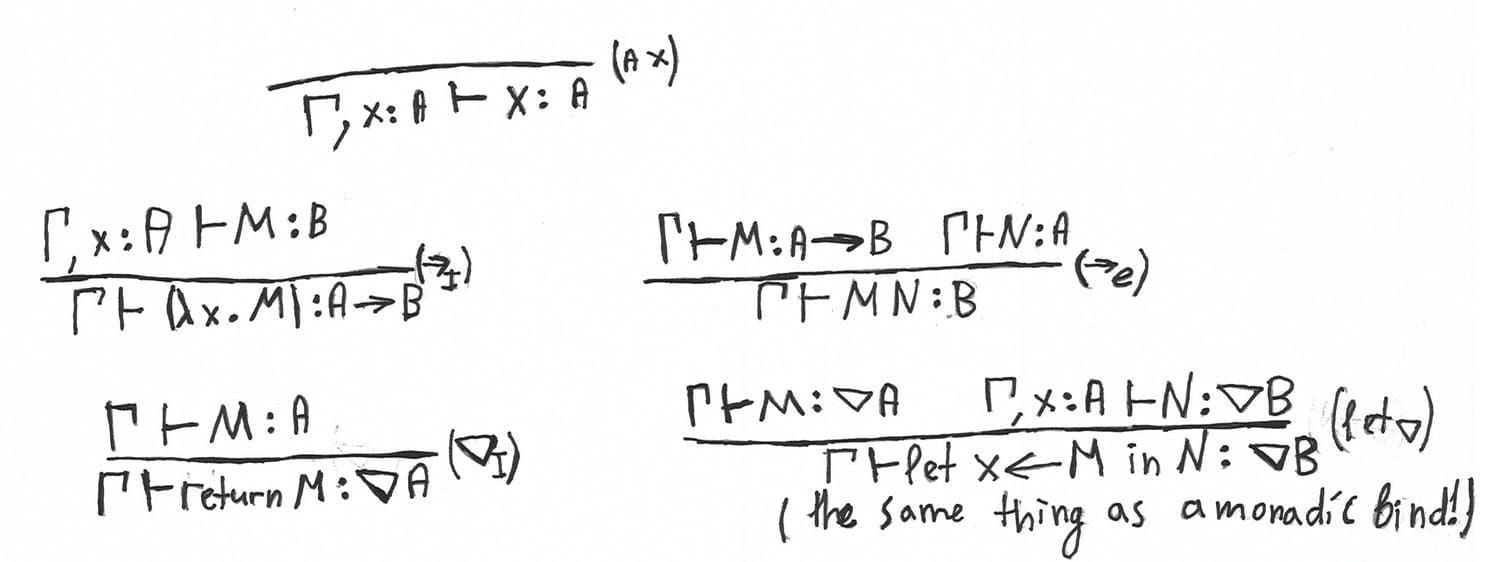
Monadic metalanguage is also studied logically, see the paper Computational Types from a Logical Perspective by P. N. Benton, G. M. Bierman, and V. de Paiva.

It is quite curious, one may consider monadic metalanguage in terms of Curry-Howard correspondence. From this perspective, this modal lambda-calculus is isomorphic to lax logic that was introduced by Robert Goldblatt in the paper called Grothendieck Topology as Geometric Modality, p.p. 131-172, where he studies modal aspects of a Grothendieck Topology, a categorical generalisation of a topological space. This logic is defined as follows:

1. Axioms of intuitionistic logic. We recall that one needs to take axioms of classical logic and replace $\neg \neg p \to p$ with $p \land \neg p \to q$
2. $\nabla (p \to q) \to (\nabla p \to \nabla q)$
3. $p \to \nabla p$
4. $\nabla \nabla p \to \nabla p$ Rules: Modus Ponens, Necessitation, and Substitution

Note that one may equivalently replace the fourth axiom with $(p \to \nabla q) \to (\nabla p \to \nabla q)$, a type of monadic bind in eyes of Haskeller.

This logic also describes syntactically so-called nucleus operator that plays a huge role in pointfree topology, a version of general topology developed within constructive mathematics. If you apparently want to get more familiar with the related concepts, you may read the book Stone Spaces by Peter Johnstone or the third volume of Handbook of Categorical Algebra (the subtitle is Sheaf Theory) by Francis Borceux. Additionally, here we also recommend the brief lecture on Topos Theory course by André Joyal, here’s the link on YouTube where the same notions are covered.

Literature overview

Let us overview some of the monographs, textbooks, and papers that we recommend to you for further study if you are interested in it.

• Basic Modal Logic by Patrick Blackburn, Maarten de Rijke and Yde Venema is one of the best introductory texts books in modal logic. This book covers such topics as relational semantics, algebraic semantics, first-order frame definability, general frames, computational aspects of modal logic and its complexity. Also, there are a lot of miscellaneous exercises that allow you to improve your mastery of the material.

• Modal Logic by Alexander Chagrov and Michael Zakharyaschev can serve the reader as a handbook in basic concepts of modal logic. This book might be considered as a more detailed version of the previous book.

• Modal Logic for Open Minds by Johan van Benthem is another introduction to modal logic. In contrast to the previous two books, Modal Logic for Open Minds is more concentrated on the variety of modal logic applications. In this book, the reader may study and build an understanding of basic spatial logic, epistemic logic, logic of time, logic in information dynamics, provability in formal arithmetic, etc. We also note that Modal Logic for Open Minds is written in accessible language and the textbook is full of humour.

• An Essay in Classical Modal Logic is a PhD thesis by written Krister Segerberg at the beginning of the 1970-s. As we told in the first part, Segerberg is one of the founders of the contemporary modal logic. One may use this thesis as a laconic introduction to modal logic, especially to such topics as Kripke semantics, neighbourhood semantics, filtrations, and completeness theorems for basic logics.

• Logics of Time and Computation by Robert Goldblatt is an introduction to modal logic but specified to tense logic and related systems that describes several dynamics and computation. The first part of the textbook is the standard introduction to basic modal logic. Further, Goldblatt studies discrete, dense, and continuous time; describes concurrent and regular computation via temporal logic with binary modalities and propositional dynamic logic. The third part covers model-theoretic aspects of predicate extensions of propositional dynamic logic.

• Mathematics of Modality is the collection of papers by Robert Goldblatt, the author of the previous book. As an alternative introduction to modal logic, I would recommend the paper called Metamathematics of Modal Logic, the very first paper from this collection. In this paper, Kripke semantics is more discussed from a model-theoretic perspective. In addition to Kripke semantics, the reader may use the paper as an introduction to categorical and algebraic aspects of modal logic. By the way, Goldblatt is one of the pioneers in Categorical Logic and he is also famous as the author of Topoi: The Categorical Analysis of Logic textbook.

• Handbook of Modal Logic, edition by Patrick Blackburn, Johan van Benthem and Frank Wolter. The title is self-explanatory. This handbook is a collection of introductory papers on diverse branches of modal logic written by well-known experts in corresponding areas. The handbook covers quite comprehensively more advanced topics and applications of modal logic in philosophy, game theory, linguistics, and program verification.

• Handbook of Spatial Logics. The title is self-explanatory to the same extent as the previous one. This handbook is a collection of papers on applications of logic in spatial structures. Here we recommend especially the paper called Modal Logics of Space written by Johan van Benthem and Guram Bezhanishvili.

• Provability Logic by Sergei Artemov and Lev Beklemishev is a comprehensive overview on the current state of affairs in provability logic, the area of modal logic that study provability of formal axiomatic theories as arithmetic and set theory. This paper has two parts. The first part is an observation of provability in arithmetical theory and its algebraic and proof-theoretical aspects. The second part is an introduction to logic of proofs that was proposed by Sergei Artemov as an extension of classical logic with proof-terms.

• Quantification in Nonclassical Logics by Dov Gabbay, Valentin Shehtman and Dmitry Skvortsov is the fundamental monograph on the semantical problems of modal first-order logic. The problem is the variety of modal predicate logics are Kripke incomplete and one has to generalise Kripke semantics of first-order modal logic to make the class of incomplete logic more narrow. Here we recommend bringing to the attention of simplicial semantics, the most general version of predicate Kripke frame based on simplicial sets.

• As we discussed, one may study weaker logics than normal ones. For that, we need to have a more general semantical framework. Such a framework is called neighbourhood semantics. Read the textbook called Neighbourhood semantics for Modal Logic by Eric Paquit to familiarise yourself with this generalisation of Kripke semantics.

• If you’re interested in temporal logic, we may recommend the textbook Temporal Logic. Mathematical Foundations and Computational Aspects by Dov M. Gabbay, Ian Hodkinson, and Mark Reynolds.

Summary

I believe the reader did a great job trying to become engaged with all this abstract material. Let us overview what we observe. We started from a philosophical motivation of modal logic and its historical roots. We got acquainted with Kripke frames, the canonical frame and model, and filtrations in the first part. In the second part, we studied some use cases. Pure modal logic is quite abstract and therefore admits miscellaneous interpretations in a variety of subject matters. Our use case observation isn’t comprehensive, it’s merely an invitation. We provided the list above for further reading if the reader considers to study modal logic herself more deeply.

I thank Gints Dreimanis and Jonn Mostovoy for editing and remarkable comments. I want to say thank you to my mate and colleague Rajab Agamov from the Department of Mathematics at Higher School of Economics for helpful conversations and the fact that he is a good lad. I’m grateful to Alexandra Voicehovska for the idea of a snake in topological illustrations. This blog post series is mostly based on the lecture course that I gave at the Computer Science Club based in the Saint-Petersburg Department of Steklov Mathematical Institute last autumn. I’m also grateful to Ilya B. Shapirovsky and Valentin B. Shehtman of the Institute for Information Transmission Problems of the Russian Academy of Sciences for discussions on the course programme.