
.png)
K-means is a data clustering approach for unsupervised machine learning that can separate unlabeled data into a predetermined number of disjoint groups of equal variance – clusters – based on their similarities.
It’s a popular algorithm thanks to its ease of use and speed on large datasets. In this blog post, we look at its underlying principles, use cases, as well as benefits and limitations.
What is k-means clustering?
K-means is an iterative algorithm that splits a dataset into non-overlapping subgroups that are called clusters. The amount of clusters created is determined by the value of k – a hyperparameter that’s chosen before running the algorithm.
.png)
How does k-means clustering work?
First, the algorithm selects k initial points, where k is the value provided to the algorithm.
Each of these serves as an initial centroid for a cluster – a real or imaginary point that represents a cluster’s center. Then each other point in the dataset is assigned to the centroid that’s closest to it by distance.
After that, we recalculate the locations of the centroids. The coordinate of the centroid is the mean value of all points of the cluster. You can use different mean functions for this, but a commonly used one is the arithmetic mean (the sum of all points, divided by the number of points).
Once we have recalculated the centroid locations, we can readjust the points to the clusters based on distance to the new locations.
The recalculation of centroids is repeated until a stopping condition has been satisfied.
Some common stopping conditions for k-means clustering are:
- The centroids don’t change location anymore.
- The data points don’t change clusters anymore.
- Finally, we can also terminate training after a set number of iterations.
To sum up, the process consists of the following steps:
- Provide the number of clusters (k) the algorithm must generate.
- Randomly select k data points and assign each as a centroid of a cluster.
- Classify data based on these centroids.
- Compute the centroids of the resulting clusters.
- Repeat the steps 3 and 4 until you reach a stopping condition.
How to choose the k value?
The end result of the algorithm depends on the number of сlusters (k) that’s selected before running the algorithm. However, choosing the right k can be hard, with options varying based on the dataset and the user’s desired clustering resolution.
The smaller the clusters, the more homogeneous data there is in each cluster. Increasing the k value leads to a reduced error rate in the resulting clustering. However, a big k can also lead to more calculation and model complexity. So we need to strike a balance between too many clusters and too few.
The most popular heuristic for this is the elbow method.
Below you can see a graphical representation of the elbow method. We calculate the variance explained by different k values while looking for an “elbow” – a value after which higher k values do not influence the results significantly. This will be the best k value to use.
.png)
Most commonly, Within Cluster Sum of Squares (WCSS) is used as the metric for explained variance in the elbow method. It calculates the sum of squares of distance from each centroid to each point in that centroid’s cluster.
We calculate this metric for the range of k values we want to test and look at the results. At the point where WCSS stops dropping significantly with each new cluster added, adding another cluster to the model won’t really increase its explanatory power by a lot. This is the “elbow,” and we can safely pick this number as the k value for the algorithm.
Watch this video to learn more about the general principles of k-means clustering and picking the k value.
What is the difference between kNN and k-means?
Since both k-nearest neighbors (kNN) and k-means clustering use a hyperparameter called k, they can be mistaken for each other. Let’s look at the differences between these machine learning algorithms.
The main difference between the two algorithms is that k-means is a clustering algorithm, while k-nearest neighbors is a classification algorithm.
K-means is an unsupervised algorithm. It divides an unlabeled set of data into clusters based on the patterns that the data exhibits. The clusters are created by the algorithm and might not map to any “human” concepts.
In contrast, kNN is a supervised algorithm. It uses a distance function to find the closest labeled points to a given unlabeled point, the classes of which are then used to classify that point. This enables you to use a previously labeled data set to label new data points. The classes used for labeling are already predetermined: there is no way to create new ones.
The k value in k-means refers to the amount of clusters that will be created by the algorithm, while the k in kNN refers to the number of points (nearest neighbors) that will be used to classify any given point.
To learn more about k-nearest neighbors, check out our post on the algorithm.
Benefits and drawbacks
To understand the advantages and disadvantages of k-means, it’s practical to compare it to hierarchical clustering.
Hierarchical clustering (hierarchical cluster analysis) is an analysis method that aims to construct a hierarchy of clusters without a predetermined number of clusters.
| K-means advantages | K-means drawbacks |
|---|---|
It is straightforward to understand and apply. |
You have to set the number of clusters – the value of k. |
| It is applicable to clusters of different shapes and dimensions. With a large number of variables, k-means performs faster than hierarchical clustering. | It’s sensitive to rescaling. For example, the outcome will be dramatically different if we rescale our data using normalization. |
| It provides tighter clusters than hierarchical clustering. | The input, such as the number of clusters in a network, significantly impacts output (value of k). |
| Clustering doesn’t work if you need the clusters to have a complex geometric shape. |
Practical applications
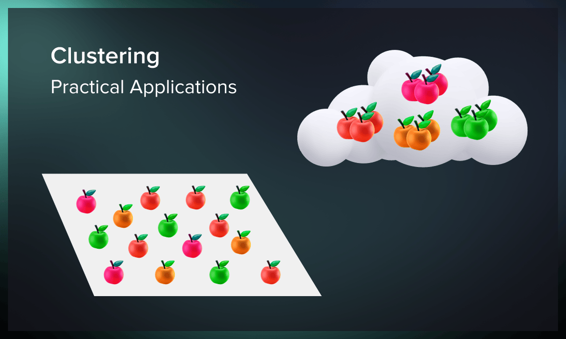
Search engines
Clustering is the foundation of many search engines that often use this technique to organize search results. To provide the user with the most accurate answer to their query, the search engine must analyze millions of unstructured pages, evaluate their content similarity, and sort the results by content relevance. After that, URLs are shown in descending order based on the assessment of hundreds of parameters, such as page content, meta tags, loading speed, usability, user behavior, etc.
K-means clustering for SE is a method for improving page ranking efficiency based on the assumption that documents with similar keywords and phrases better match search queries.
To evaluate the similarity of documents, search engines break down each record into individual words, phrases, and combinations of words. Since not all words are equally important, elements such as prepositions and articles are excluded from the analysis. The remaining content is ranked according to its relevance to the user’s query, previous searches, frequency of use in the natural language (TF-IDF matrix of features), and some other metrics.
Anomaly detection for business analysis
K-means clustering can be used to identify data points that are different from all others in the same dataset (outliers). These could be abnormal time values, non-typical user behavior, inconsistent experiment results, etc. One example is the analysis of repetitive transactions in the financial market. The algorithm can separate a group of users with suspicious behavior who conduct too many transactions in a short time and alert the bank or financial organization of possible fraud.
Real estate
The k-means clustering algorithm can effectively group properties with similar non-spatial characteristics affecting the value of the premises. This categorization method helps elaborate tax maps, improve property resource management, and facilitate decision making.
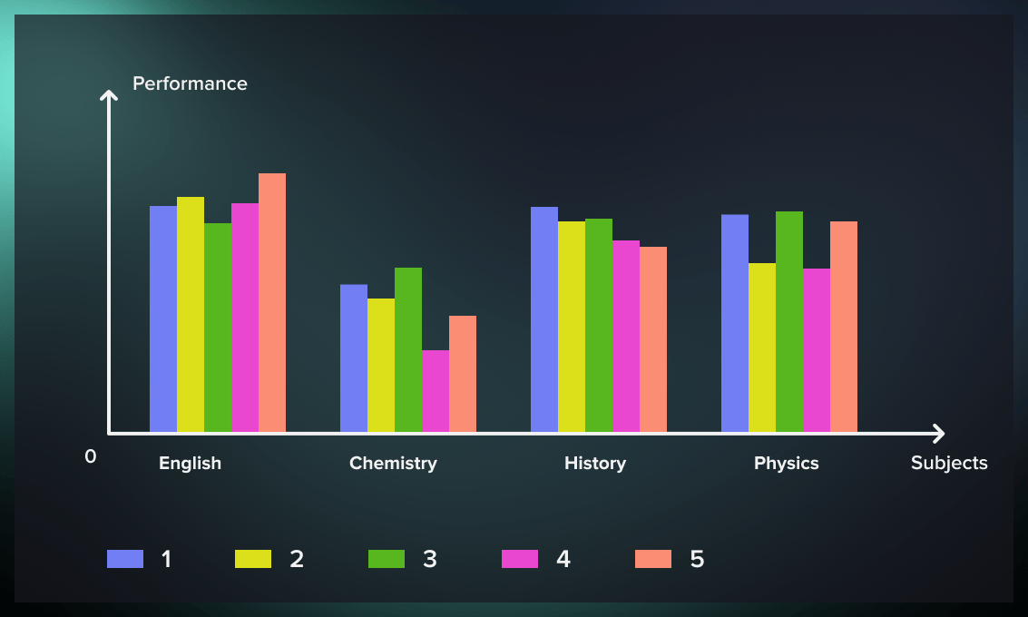
Measuring academic results
K-means can group students based on their test scores and preliminary assessments, providing insight into the effectiveness of teaching methods or student motivation. Student clustering gives an educational institution objective metrics that can help understand how to improve academic performance in the long and short term.
Medical diagnosis
In healthcare, k-means is used to develop intelligent medical decision support systems, particularly in treating liver diseases. The main benefit of using k-means clustering in medical diagnosis is that we can recognize a particular disease earlier by clustering the patients with similar symptoms. This unsupervised method supports the doctor’s research when the disease has not yet been identified because of a lack of data. In contrast, the ML model assigns a patient to a cluster based on the available analysis results, providing a direction for further investigation.
Serokell has successfully worked with biotech companies. Find out about the services we offer as a biotech software developer.
Customer segmentation
In retail, the simplest segmentation can be done based on demographics similarities. An unsupervised machine algorithm, such as k-means for cluster analysis, allows us to divide customers into groups with similar behavioral patterns and consumer preferences. With this information, it is possible to customize the ads, send targeted newsletters, offer special coupons to certain categories, and stimulate rare buyers with unique offers tailored to their preferences.
Image clustering
Clustering is one of the essential stages of image recognition. Suppose we want to detect a chair or a person in an indoor image. In that case, we can use image clustering to separate backgrounds and important elements and analyze each object separately. K-means fulfills this task quickly and efficiently.
Example: k-means clustering with scikit-learn
As an example, we’ll apply k-means clustering to medical data. We’ll use the diabetes dataset and the k-means algorithm available in the sklearn package.
from sklearn.cluster import KMeans
from sklearn import datasets
from sklearn.utils import shuffle

diabetes = datasets.load_diabetes()
The dataset gives us data on 442 diabetes patients with variables like age, sex, body mass index (BMI), blood pressure, and blood serum measurements. Suppose we want to divide the patients into groups for determining certain risk groups.
For simplicity, we’ll only work with the first three columns: sex, age, and body mass index (BMI).
X = diabetes.data[:,:3]
y = diabetes.target
names = diabetes.feature_names[:3]
X, y = shuffle(X, y, random_state=42)
For the division to be representative, we need to find the optimal number of clusters (patient groups) before clustering.
We can do it with the elbow method described in this article. We’ll run k-means with cluster numbers from 1 to 50 and calculate Euclidean distances between points and cluster centroids. By summarizing these distances, we’ll get the within-cluster squared error (WSS).
The number of clusters where this error stops to decrease dramatically is the optimal “elbow” we want to find.
from tqdm.notebook import tqdm as tqdm
def calculate_WSS(points, kmax):
  sse = []
  for k in tqdm(range(1, kmax+1)):
    kmeans = KMeans(n_clusters = k).fit(points)
    centroids = kmeans.cluster_centers_
    pred_clusters = kmeans.predict(points)
    curr_sse = 0

    for i in range(len(points)):
      curr_center = centroids[pred_clusters[i]]
      curr_sse += (points[i, 0] - curr_center[0]) ** 2 + (points[i, 1] - curr_center[1]) ** 2

    sse.append(curr_sse)
  return sse
sse = calculate_WSS(X, 50)
We can plot the results on a chart.
import matplotlib.pyplot as plt
import matplotlib as mpl

%matplotlib inline
plt.plot(sse)
plt.grid()
plt.title('Sum of squared errors within centroids dependent on number of clusters')
plt.xlabel('N Clusters')
plt.ylabel('Sum of squared errors')
plt.show()
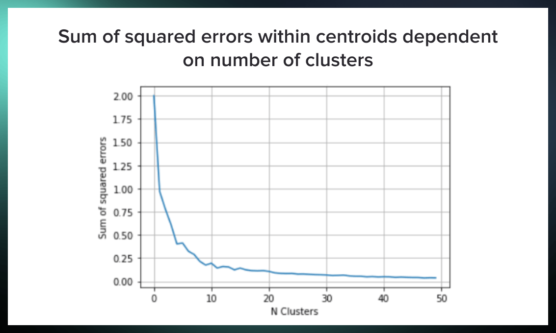
From the chart above, it’s clear that the “elbow” is somewhere around the k value of 10. So let’s run k-means with 10 clusters.
model = KMeans(n_clusters=10, random_state=42)
diabetes_kmeans = model.fit(X)

fig = plt.figure(figsize=(20, 10))
ax1 = fig.add_subplot(1, 2, 1, projection='3d')
ax1.scatter(X[:, 0], X[:, 1], X[:, 2],
            c=diabetes_kmeans.labels_.astype(float),
           edgecolor="k", s=150, cmap=plt.get_cmap('Paired'))
ax1.view_init(20, -50)
ax1.set_xlabel(names[0], fontsize=12)
ax1.set_ylabel(names[1], fontsize=12)
ax1.set_zlabel(names[2], fontsize=12)
ax1.set_title("K-Means Clusters for the Diabetes Dataset", fontsize=12)

ax2 = fig.add_subplot(1, 2, 2, projection='3d')
ax2.scatter(X[:, 0], X[:, 1], X[:, 2],
            c=y, edgecolor="k", s=150,
            cmap=plt.get_cmap('Greys'))
ax2.view_init(20, -50)
ax2.set_xlabel(names[0], fontsize=12)
ax2.set_ylabel(names[1], fontsize=12)
ax2.set_zlabel(names[2], fontsize=12)
ax2.set_title("Diabetes progression", fontsize=12)
fig.show()
Now we can analyze the results of clustering. An important note is that the dataset was normalized beforehand, so the values for age, sex, and BMI are not absolute but percentage deviations from the mean.
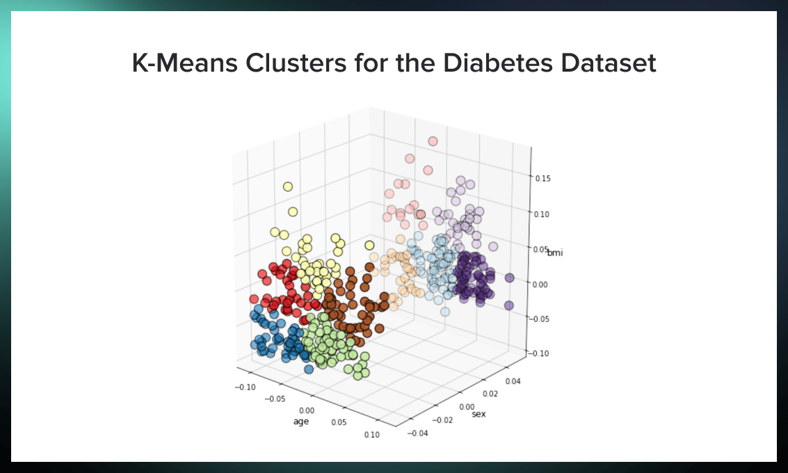
The first figure shows the clusters found. The main subdivision is by sex, with five groups for women and men. The bright dots on the left represent women, while the pale dots on the right represent men.
Women can be divided into five groups:
- younger patients with low BMI (blue);
- older patients with low BMI (green);
- younger patients with average BMI (red);
- older patients with average BMI (brown);
- middle-aged women with high BMI (yellow).
For men, we have the following groups:
- young patients with low BMI (pale brown);
- middle-aged patients with low to average BMI (pale blue);
- older patients with low BMI (purple);
- older patients with high BMI (pale purple);
- younger patients with high BMI (pale red).
The target variable for the dataset contains blood test results showing which patients have developed diabetes and how pronounced their condition is. You can see a plot with this value in the second plot.
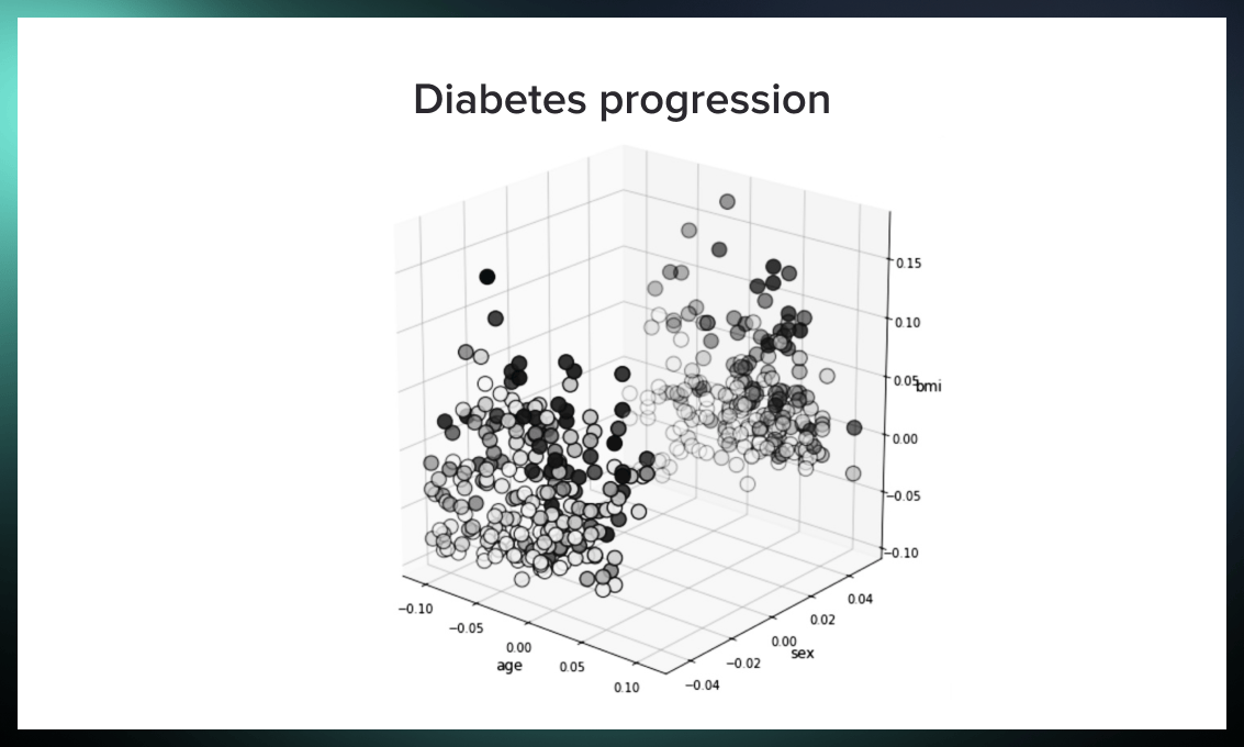
The most severe cases are colored black, while the milder cases are gray. For both women and men, we can deduce that the groups with high BMI and older age are most at risk. They are grouped in clusters of yellow, brown, light, red, and light purple.
Conclusion: why is the method so popular?
K-means is the fastest unsupervised machine learning algorithm to break down data points into groups even when very little information is available. Thanks to its high speed, K-means clustering is a good choice for large datasets. Simple and flexible, it’s also the optimal algorithm to get started with clustering.
All these features make it effective for multiple industries, including scientific research, business analysis, archive management, search engines, etc.

.jpg)
.jpg)


.jpg)