K-Nearest Neighbors Algorithm for ML

The k-nearest neighbors (kNN) algorithm is a simple tool that can be used for a number of real-world problems in finance, healthcare, recommendation systems, and much more. This blog post will cover what kNN is, how it works, and how to implement it in machine learning projects.

What is the k-nearest neighbors classifier?

The k-nearest neighbors classifier (kNN) is a non-parametric supervised machine learning algorithm. It’s distance-based: it classifies objects based on their proximate neighbors’ classes. kNN is most often used for classification, but can be applied to regression problems as well.

What is a supervised machine learning model? In a supervised model, learning is guided by labels in the training set. For a better understanding of how it works, check out our detailed explanation of supervised learning principles.

Non-parametric means that there is no fine-tuning of parameters in the training step of the model. Although k can be considered an algorithm parameter in some sense, it’s actually a hyperparameter. It’s selected manually and remains fixed at both training and inference time.

The k-nearest neighbors algorithm is also non-linear. In contrast to simpler models like linear regression, it will work well with data in which the relationship between the independent variable (x) and the dependent variable (y) is not a straight line.

What is k in k-nearest neighbors?

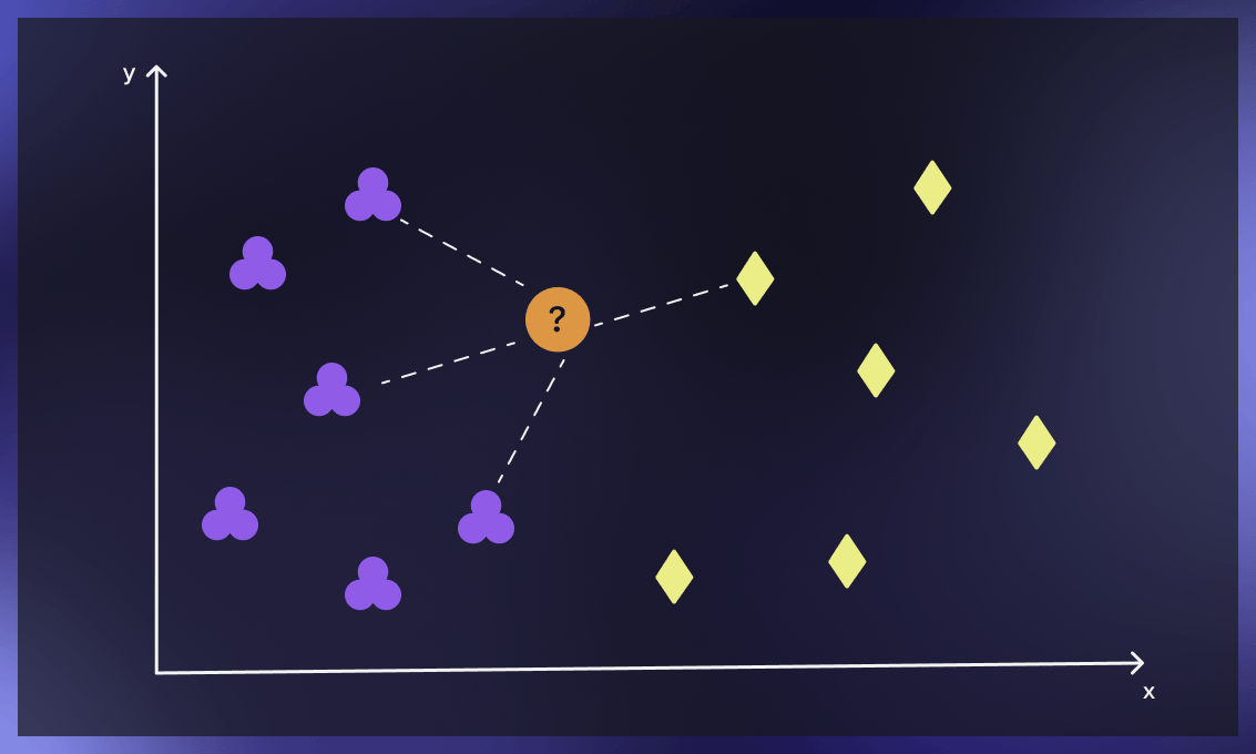
The parameter k in kNN refers to the number of labeled points (neighbors) considered for classification. The value of k indicates the number of these points used to determine the result. Our task is to calculate the distance and identify which categories are closest to our unknown entity.

How does the kNN classification algorithm work?

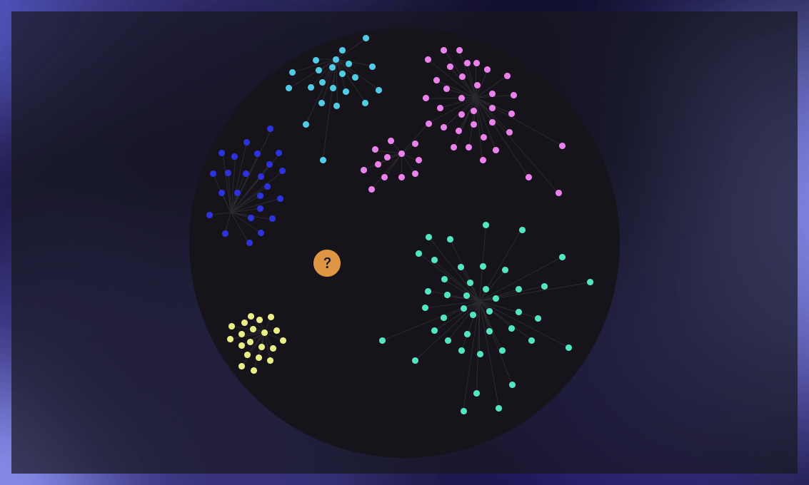
The main concept behind k-nearest neighbors is as follows. Given a point whose class we do not know, we can try to understand which points in our feature space are closest to it. These points are the k-nearest neighbors. Since similar things occupy similar places in feature space, it’s very likely that the point belongs to the same class as its neighbors. Based on that, it’s possible to classify a new point as belonging to one class or another.

The kNN algorithm step-by-step

Provide a training set

A training set is a set of labeled data that’s used for training a model. You can create the training set by manually labeling data or use the labeled databases available in public resources, like this one. A good practice is to use around 75% of the available data for training and 25% as the testing set.

Find k-nearest neighbors

Finding k-nearest neighbors of a record means identifying those records which are most similar to it in terms of common features. This step is also known as similarity search or distance calculation.

Classify points

For classification problems, the algorithm assigns a class label based on a majority vote, meaning that the most frequent label that occurs in neighbors is applied. For regression problems, the average is used to identify the k nearest neighbors.

After the completion of the above steps, the model provides the results. Note that for classification problems, we use discrete values, so the output would be descriptive, for example “likes bright colors”.

For regression problems, continuous values are applied, meaning that the output would be a floating-point number.

We can evaluate the accuracy of the results by looking at how close the model’s predictions and estimates match the known classes in the testing set.

How to determine the k value in the k-neighbors classifier?

The optimal k value will help you to achieve the maximum accuracy of the model. This process, however, is always challenging.

The simplest solution is to try out k values and find the one that brings the best results on the testing set. For this, we follow these steps:

1. Select a random k value. In practice, k is usually chosen at random between 3 and 10, but there are no strict rules. A small value of k results in unstable decision boundaries. A large value of k often leads to the smoothening of decision boundaries but not always to better metrics. So it’s always about trial and error.

2. Try out different k values and note their accuracy on the testing set.

3. Сhoose k with the lowest error rate and implement the model.

Picking k in more complicated cases

In the case of anomalies or a large number of neighbors closely surrounding the unknown point, we need to find different solutions for calculating k that are both time- and cost-efficient.

The main limitations are related to computational resources: the more objects there are in the dataset, the higher the cost of appropriate k selection is. Moreover, with big datasets, we usually work in a multiparameter optimization setup. Our goal here is not only to maximize model quality by choosing the right k in meta-training but also to achieve faster model inference. If k is bigger, more inference time is needed, which could pose a problem in large data sets.

Below we present some advanced methods for selecting k that are suitable for these cases.

1. Square root method

The optimal K value can be calculated as the square root of the total number of samples in the training dataset. Use an error plot or accuracy plot to find the most favorable K value. KNN performs well with multi-label classes, but in case of the structure with many outliers, it can fail, and you’ll need to use other methods.

2. Cross-validation method (Elbow method)

Begin with k=1, then perform cross-validation (5 to 10 fold – these figures are common practice as they provide a good balance between the computational efforts and statistical validity), and evaluate the accuracy. Keep repeating the same steps until you get consistent results. As k goes up, the error usually decreases, then stabilizes, and then grows again. The optimal k lies at the beginning of the stable zone.

You can watch a detailed explanation of this methods below.

How is the k-distance calculated?

K-distance is the distance between data points and a given query point. To calculate it, we have to pick a distance metric.

Some of the most popular metrics are explained below.

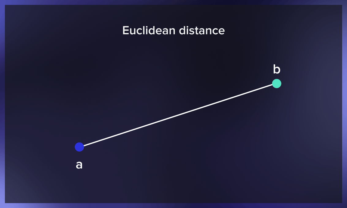
Euclidean distance

The Euclidean distance between two points is the length of the straight line segment connecting them. This most common distance metric is applied to real-valued vectors.

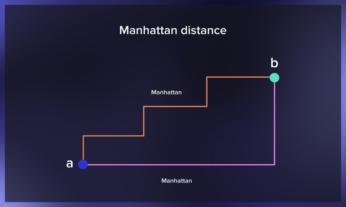
Manhattan distance

The Manhattan distance between two points is the sum of the absolute differences between the x and y coordinates of each point. Used to measure the minimum distance by summing the length of all the intervals needed to get from one location to another in a city, it’s also known as the taxicab distance.

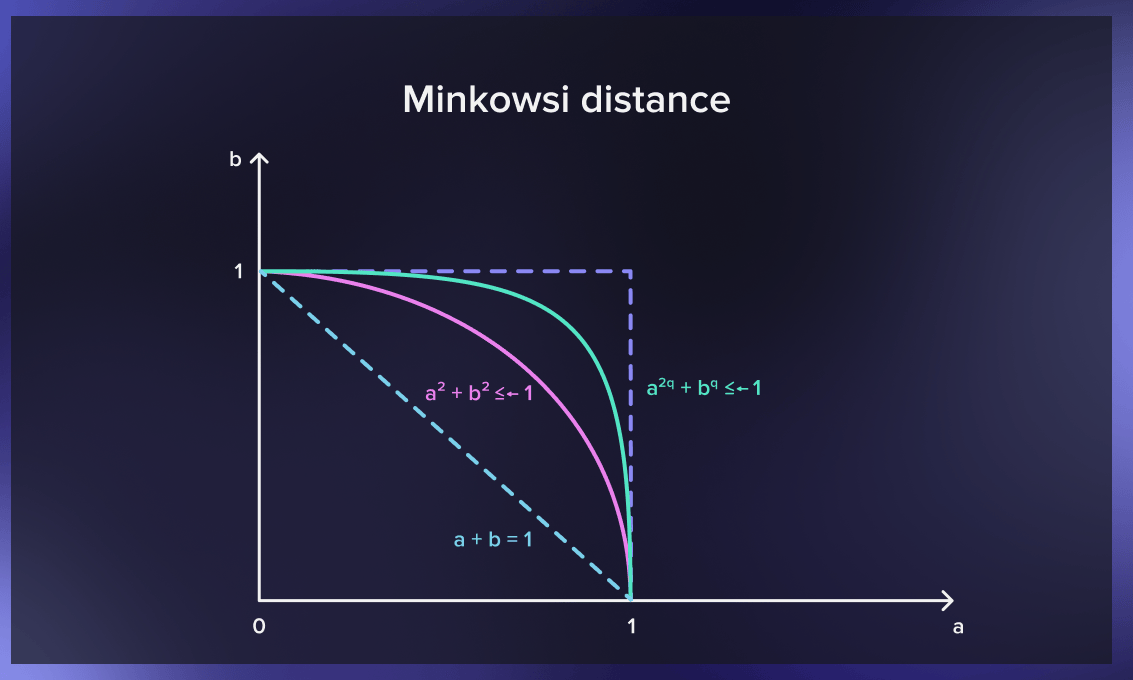
Minkowski distance

Minkowski distance generalizes the Euclidean and Manhattan distances. It adds a parameter called “order” that allows different distance measures to be calculated. Minkowski distance indicates a distance between two points in a normed vector space

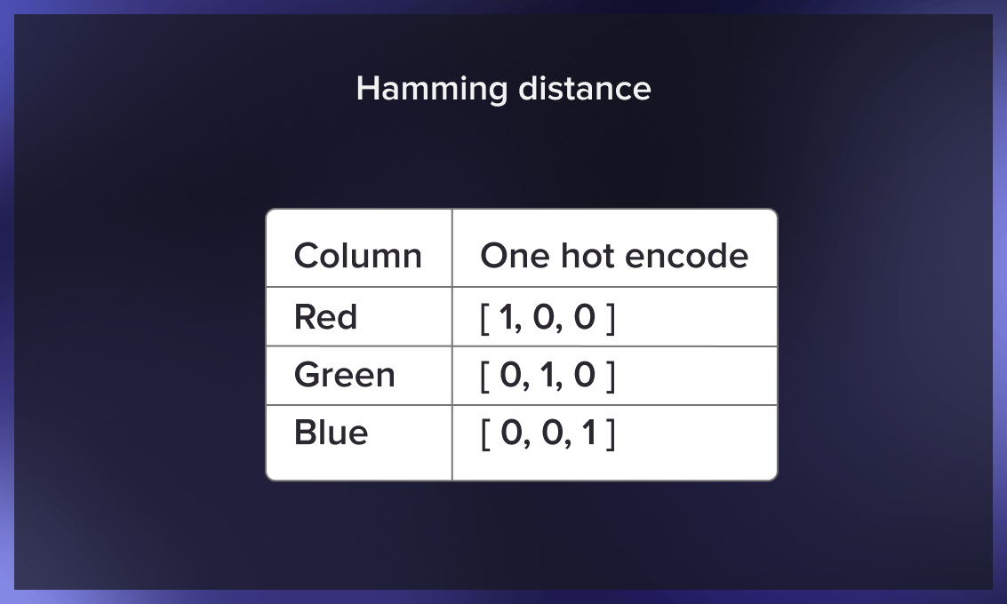
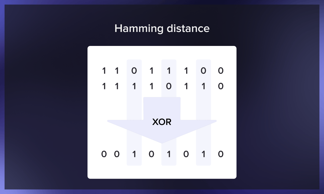
Hamming distance

Hamming distance is used to compare two binary vectors (also called data strings or bitstrings). To calculate it, data first has to be translated into a binary system.

K-nearest neighbors with Python

Let’s examine the functioning of the classifier in a practical setting using Python.

First steps

First, we need to generate data on which we’ll run the classifier:

import numpy as np
from typing import Tuple

def generate_data(center_scale: float, cluster_scale: float, class_counts: np.ndarray,
                  seed: int = 42) -> Tuple[np.ndarray, np.ndarray]:
    # Fix a seed to make experiment reproducible
    np.random.seed(seed)
    points, classes = [], []
    for class_index, class_count in enumerate(class_counts):
        # Generate the center of the cluster and its points centered around it
        current_center = np.random.normal(scale=center_scale, size=(1, 2))
        current_points = np.random.normal(scale=cluster_scale, size=(class_count, 2)) + current_center
        # Assign them to the same class and add those points to the general pool
        current_classes = np.ones(class_count, dtype=np.int64) * class_index
        points.append(current_points)
        classes.append(current_classes)
    # Concatenate clusters into a single array of points
    points = np.concatenate(points)
    classes = np.concatenate(classes)
    return points, classes

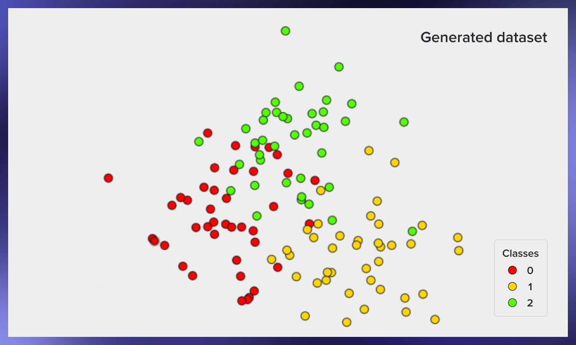
points, classes = generate_data(2, 0.75, [40, 40, 40], seed=42)

To plot the generated data, you can run the following code:

import matplotlib.pyplot as plt
plt.style.use('bmh')

def plot_data(points: np.ndarray, classes: np.ndarray) -> None:
    fig, ax = plt.subplots(figsize=(5, 5), dpi=150)
    scatter = ax.scatter(x=points[:, 0], y=points[:, 1], c=classes, cmap='prism', edgecolor='black')
    # Generate a legend based on the data and plot it
    legend = ax.legend(*scatter.legend_elements(), loc="lower left", title="Classes")
    ax.add_artist(legend)
    ax.set_title("Generated dataset")
    ax.set_xticks([])
    ax.set_yticks([])
    plt.show()

plot_data(points, classes)

Here’s an example of the resulting image from this code:

How to split training and testing samples

Now we have a labeled set of objects, each of which is assigned to a class. We need to split this set into two parts: a training set and a test set. The following code is used for this:

from sklearn.model_selection import train_test_split

points_train, points_test, classes_train, classes_test = train_test_split(
    points, classes, test_size=0.3
)

Classifier implementation

Now that we have a training sample, we can implement the classifier algorithm:

from collections import Counter

def classify_knn(
    points_train: np.ndarray,
    classes_train: np.ndarray,
    points_test: np.ndarray,
    num_neighbors: int
) -> np.ndarray:
    classes_test = np.zeros(points_test.shape[0], dtype=np.int64)
    for index, test_point in enumerate(points_test):
        # Compute Euclidean norm between the test point and the training dataset
        distances = np.linalg.norm(points_train - test_point, ord=2, axis=1)
        # Collect the closest neighbors indices based on the distance calculated earlier
        neighbors = np.argpartition(distances, num_neighbors)[:num_neighbors]
        # Get the classes of those neighbors and assign the most popular one to the test point
        neighbors_classes = classes_train[neighbors]
        test_point_class = Counter(neighbors_classes).most_common(1)[0][0]
        classes_test[index] = test_point_class
    return classes_test

classes_predicted = classify_knn(points_train, classes_train, points_test, 3)

Examples of execution

Now we can evaluate how well our classifier works. To do this, we generate data, split it into a training set and a test set, classify the objects in the test set, and compare the actual value of the classes in the test set to the value resulting from the classification:

def accuracy(classes_true, classes_predicted):
    return np.mean(classes_true == classes_predicted)

knn_accuracy = accuracy(classes_test, classes_predicted)

#> knn_accuracy
#  0.8055555555555556

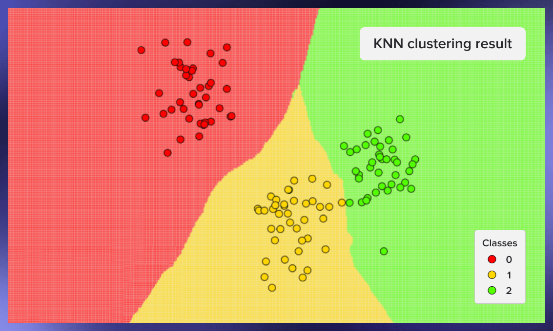
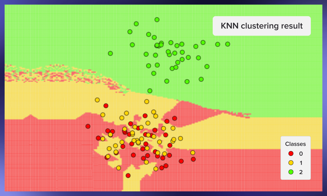
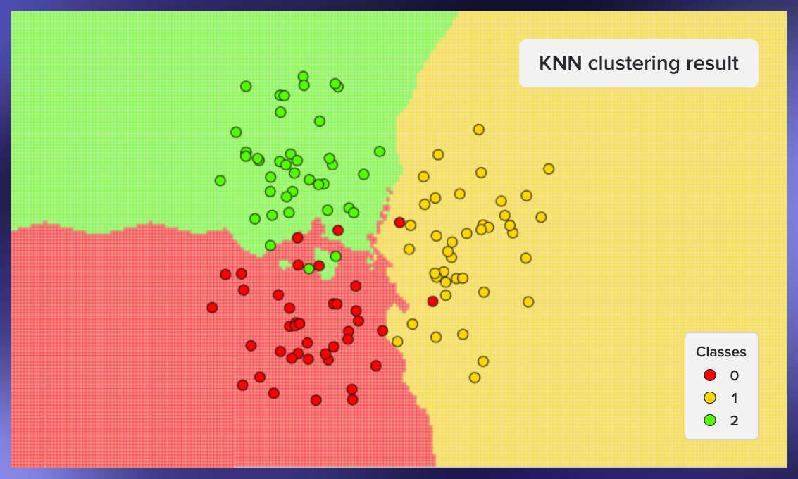
Now we can graphically show the work of the classifier. In the pictures below we used 3 classes with 40 elements each, the value of k for the algorithm was set equal to three.

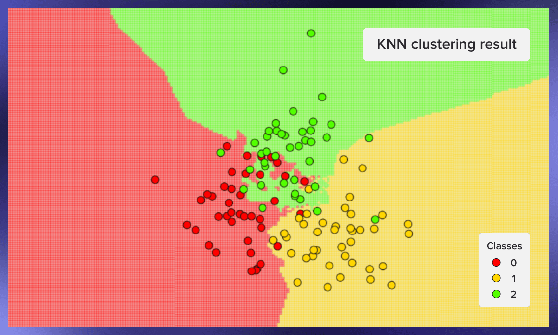
For creating these graphics, we can use the following code:

def knn_prediction_visualisation(
    points: np.ndarray,
    classes: np.ndarray,
    num_neighbors: int
) -> None:
    x_min, x_max = points[:, 0].min() - 1, points[:, 0].max() + 1
    y_min, y_max = points[:, 1].min() - 1, points[:, 1].max() + 1
    step = 0.05


    # Prepare a mesh grid of the plane to cluster
    mesh_test_x, mesh_test_y = np.meshgrid(
        np.arange(x_min, x_max, step), np.arange(y_min, y_max, step)
    )
    points_test = np.stack([mesh_test_x.ravel(), mesh_test_y.ravel()], axis=1)
    # Predict clusters and prepare the results for the plotting
    classes_predicted = classify_knn(points, classes, points_test, num_neighbors)
    mesh_classes_predicted = classes_predicted.reshape(mesh_test_x.shape)


    # Plot the results
    fig, ax = plt.subplots(figsize=(5, 5), dpi=150)
    ax.pcolormesh(mesh_test_x, mesh_test_y, mesh_classes_predicted,
                  shading='auto', cmap='prism', alpha=0.4)
    scatter = ax.scatter(x=points[:, 0], y=points[:, 1], c=classes,
                         edgecolors='black', cmap='prism')
    legend = ax.legend(*scatter.legend_elements(), loc="lower left", title="Classes")
    ax.set_title("KNN clustering result")
    ax.set_xticks([])
    ax.set_yticks([])


    plt.show()

knn_prediction_visualisation(points, classes, 3)

Here are some other examples of clustering – first from the seed 59, second from the seed 0xdeadbeef, third from the seed 777:

Pros and cons of kNN

The main advantage of kNN is that it’s fast to develop and simple to interpret:

• It can be used for both classification and regression problems.
• kNN is easy to understand and implement and does not require a training period.
• The researcher does not need to have initial assumptions about how similar or dissimilar two examples are.
• K-nearest neighbors only builds a model once a query is performed on the dataset.
• The algorithm can be quickly and effectively paralleled in inference time, which is especially useful for large datasets.

However, the algorithm has its weaknesses too.

• kNN is more memory-consuming than other classifying algorithms as it requires you to load the entire dataset to run the computation, which increases computation time and costs.
• The k-nearest neighbors algorithm performs worse on more complex tasks such as text classification.
• It requires feature scaling (normalization and standardization) in each dimension.

Practical applications

K-nearest neighbors method for сar manufacturing

An automaker has designed prototypes of a new truck and sedan. To determine their chances of success, the company has to find out which current vehicles on the market are most similar to the prototypes. Their competitors are their "nearest neighbors.” To identify them, the car manufacturer needs to input data such as price, horsepower, engine size, wheelbase, curb weight, fuel tank capacity, etc., and compare the existing models. The kNN algorithm classifies complicated multi-featured prototypes according to their closeness to similar competitors’ products.

kNN in E-commerce

K-nearest neighbors is an excellent solution for cold-starting an online store recommendation system, but with the growth of the dataset more advanced techniques are usually needed. The algorithm can select the items that specific customers would like or predict their actions based on customer behavior data. For example, kNN will quickly tell whether or not a new visitor will likely carry out a transaction.

kNN application for education

Another kNN application is classifying groups of students based on their behavior and class attendance. With the help of the k-nearest neighbors analysis, it is possible to identify students who are likely to drop out or fail early. These insights would allow educators and course managers to take timely measures to motivate and help them master the material.

Takeaways

The kNN algorithm is popular, effective, and relatively easy to implement and interpret. It can efficiently solve classification and regression tasks for complicated multivariate cases. Despite the emergence of many advanced alternatives, it maintains its position among the best ML classifiers.