A Guide to F1 Score

Effective evaluation metrics are crucial in assessing the performance of machine learning models. One of such metrics is the F1 score, which is widely used for classification problems, information retrieval, and NLP tasks.

In this blog post, we’ll explore the foundational concepts of the F1 score, discuss its limitations, and look at use cases across diverse domains.

What is the F1 score in machine learning?

The performance of ML algorithms is measured using a set of evaluation metrics, with model accuracy being among the commonly used ones.

Accuracy calculates the number of correct predictions made by a model across the entire dataset, which is valid when the dataset classes are balanced in size. In the past, accuracy was the sole criterion for comparing machine learning models.

But real-world datasets often exhibit heavy class imbalance, rendering the accuracy metric impractical. For instance, in a binary class dataset with 90 samples in class 1 and 10 samples in class 2, a model that consistently predicts “class 1” would still achieve 90% accuracy. But can we consider this model a good predictor?

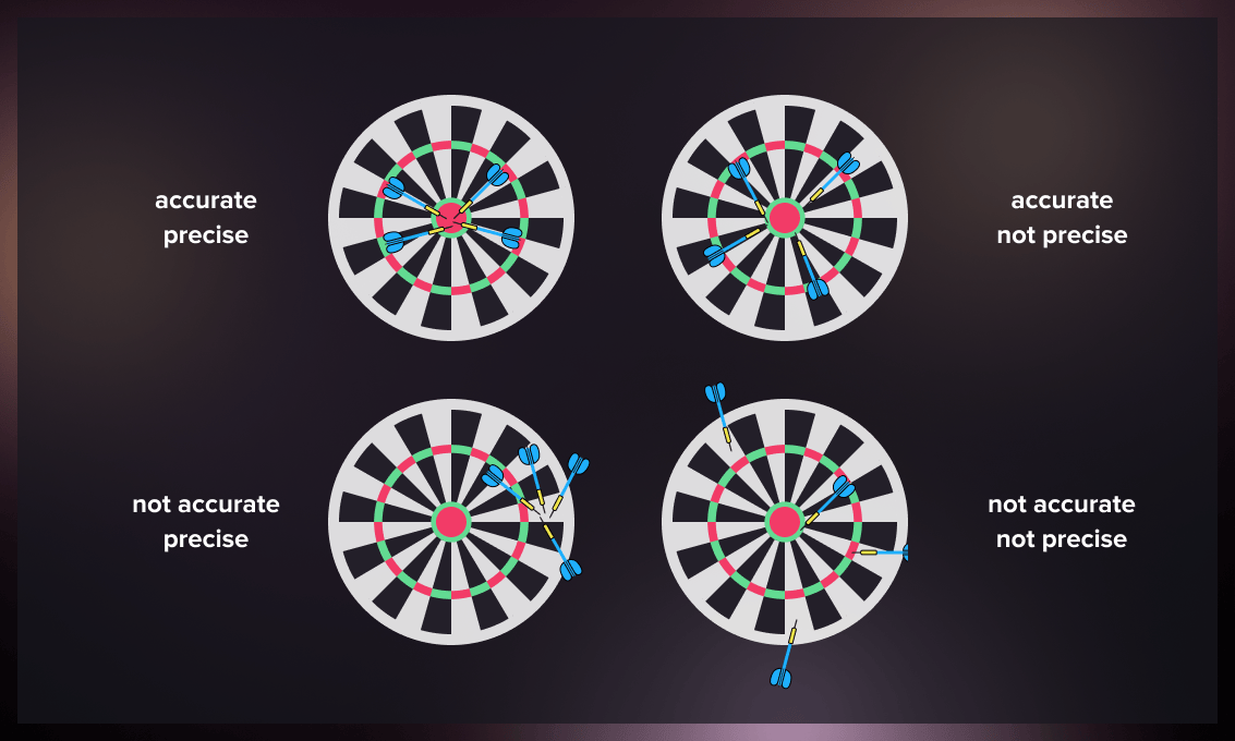
Today data scientists use the precision measure alongside accuracy. While accuracy assesses the proximity to the actual value of the measurement, precision indicates the proximity of the predicted values to each other.

The bullseye analogy is commonly used to illustrate the difference between accuracy and precision. Imagine you are throwing darts at a bullseye with the goal of achieving both accuracy and precision, meaning you want to consistently hit the bullseye. Accuracy refers to landing your throws near the bullseye, but not necessarily hitting it every time. On the other hand, precision means your throws cluster closely together, but they may not be near the bullseye. However, when you are both accurate and precise, your darts will consistently hit the bullseye.

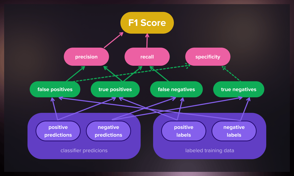
An alternative evaluation metric in machine learning is the F1 score, which assesses the predictive ability of a model by examining its performance on each class individually rather than considering overall performance like accuracy does. The F1 score combines two competing metrics, precision and recall.

Precision and recall

First, let’s understand precision and recall in the context of a binary class dataset with “positive” and “negative” labels.

• Precision quantifies the proportion of correct “positive” predictions made by the model.
• Recall measures the proportion of positive class samples the model correctly identifies.

Consider an email spam filter (a binary classification problem), where “spam” is the positive class and “not spam” is the negative class.

Precision: Let’s say out of 100 emails that the filter marks as spam, 95 are indeed spam, and 5 are not. In this case, the precision of the spam filter is 95% (95 out of 100), indicating high accuracy in its positive (“spam”) predictions.

Recall: Now, suppose there are 200 actual spam emails, and the filter only catches 150. The recall of the spam filter would be 75% (150 out of 200), meaning it was able to detect 75% of the total spam emails.

Trade-off between precision and recall

Often in machine learning models, there’s a trade-off between precision and recall. Improving precision may lead to a decrease in recall, and vice versa. As a model strives to catch all positive instances (to increase recall), it may end up wrongly classifying some negative instances as positive, thereby reducing precision. Conversely, as a model becomes more conservative in predicting positives to increase precision, it may miss some actual positive instances, lowering recall.

So in the spam filter example, if we want the filter to catch all spam emails (increase recall), it might result in more non-spam emails being wrongly classified as spam (lower precision). On the other hand, making the filter stricter to minimize non-spam emails marked as spam (increase precision) might cause it to miss some actual spam emails (lower recall).

Ideally, we aim to maximize both precision and recall to obtain the perfect classifier.

Watch this video to get a better understanding of precision and recall:

How to calculate the F1 score

The F1 score blends precision and recall using their harmonic mean. Maximizing for the F1 score implies simultaneously maximizing for both precision and recall.

The mathematical formula for the F1 score is as follows:

$$F1 = 2 * \frac {Precision * Recall} {Precision + Recall}$$

Unlike the arithmetic mean, the harmonic mean tends to be closer to the smaller number in a pair. Thus, the F1 score will only be high if both precision and recall are high, ensuring a good balance of both.

Detailed step-by-step guide on calculating F1 score

1. Calculate True Positives (TP): These are the correctly predicted positive values. It means the actual class was positive, and the model prediction is also positive.
2. Calculate False Positives (FP): These are values for which the actual class is negative, but the predicted one is positive.
3. Calculate False Negatives (FN): These are values for which the actual class is positive, but the predicted one is negative.
4. Calculate precision: TP divided by the sum of TP and FP.
5. Calculate recall: TP divided by the sum of TP and FN.
6. Finally, calculate the F1 score using the following formula: 2 \* (precision \* recall) / (precision + recall)

Let’s take an example of a disease detection test where:

• True Positives (TP) = 100 (The test correctly identified 100 patients with the disease)
• False Positives (FP) = 10 (The test incorrectly identified 10 healthy patients as having the disease)
• False Negatives (FN) = 20 (The test incorrectly identified 20 patients with the disease as healthy)

Step 1: Calculate precision

$$Precision = TP / (TP + FP) = 100 / (100 + 10) = 0.909$$

Step 2: Calculate recall

$$Recall = TP / (TP + FN) = 100 / (100 + 20) = 0.833$$

Step 3: Calculate F1 score

$$F1 = 2 \ (Precision * Recall) / (Precision + Recall) = 2 * (0.909 \ 0.833) / (0.909 + 0.833) = 0.869$$

So the F1 score of the disease detection model in this example is 0.869.

What does the F1 score tell you?

In a binary classification model, a large F1 score of 1 indicates excellent precision and recall, while a low score indicates poor model performance.

Interpreting the F1 score depends on the specific problem and context at hand. In general, a higher F1 score suggests better model performance. However, what constitutes a “good” or “acceptable” F1 score varies based on factors such as the domain, application, and consequences of errors.

For instance, in a medical diagnosis task where missing a disease is more critical than falsely diagnosing it, a high recall score (even at the expense of precision) becomes more important. In this case, a higher F1 score would be desirable. Conversely, in a spam filtering task where misclassifying a legitimate email as spam is more detrimental than letting a spam email through, a high precision score (even at the expense of recall) is more important. Thus, a higher F1 score would be desired in this scenario.

What is considered a good F1 score?

As a general guideline, an F1 score of 0.7 or higher is often considered good. But again, you need to consider the specific context. Some applications may necessitate a higher F1 score, especially if both precision and recall are critical.

The F1 score should be assessed alongside other metrics and factors, including dataset characteristics, problem complexity, and the cost associated with misclassification.

Low F1 score

A low F1 score indicates poor overall performance of a binary classification model and can be attributed to various factors, including:

1. Imbalanced data: In case of an imbalanced dataset, with one class being represented significantly more frequently than the other, the model may struggle to learn to distinguish the minority class, resulting in poor performance and a low score.
2. Insufficient data: Inadequate dataset size or insufficient representative examples of each class can hinder the model’s ability to learn a robust representation.
3. Inappropriate model selection: Score might be low if the chosen model is not suitable for the specific task or if it is not properly tuned.
4. Inadequate features: If the selected features fail to capture the relevant information for the task, the model may struggle to learn meaningful patterns from the data.

To improve the F1 score, it is necessary to determine the underlying causes of poor performance and take appropriate steps to address them. For example, if the dataset is imbalanced, you can apply oversampling or undersampling to balance the classes. If the model is unsuitable or poorly tuned, exploring alternative models or performing hyperparameter tuning may be beneficial. Additionally, inadequate features can be addressed through feature engineering or selection to identify more relevant features for the task at hand.

High F1 score

A high F1 score indicates the strong overall performance of a binary classification model. It signifies that the model can effectively identify positive cases while minimizing false positives and false negatives.

You can achieve a high F1 score using the following techniques:

1. High-quality training data: A high-quality dataset that accurately represents the problem being solved can significantly improve the model’s performance.
2. Appropriate model selection: Selecting a model architecture well-suited for the specific problem can enhance the model’s ability to learn and identify patterns within the data.
3. Effective feature engineering: Choosing or creating informative features that capture relevant information from the data can enhance the model’s learning capabilities and generalization.
4. Hyperparameter tuning: Optimizing the model’s hyperparameters through careful tuning can improve its performance.

Note that a high F1 score does not guarantee flawless performance, and the model may still make errors. Also, a slightly lower F1 score may still be acceptable in some instances if it appropriately balances the trade-off between precision and recall based on the specific task requirements.

How to compute the F1 score in Python?

The F1 score can be easily calculated in Python using the “f1_score” function from the scikit-learn package. This function requires three main arguments: the true labels, the predicted labels, and an “average” parameter.

When dealing with a binary-class dataset, the “binary” mode of the average parameter is used to obtain the class-specific F1 score. The “micro,” “macro,” and “weighted” modes are used for datasets with any number of classes, providing different averaging schemes for calculating the scores. Using “None” as the average parameter returns all individual class-wise F1 scores.

To obtain a comprehensive list of metrics in one go, you can utilize the “classification_report” function from scikit-learn.

Generalized Fβ-score formula

Adjusted F-score enables us to assign a higher weight to precision and/or recall if they are crucial for our study. The formula for the adjusted F-score is as follows:

$$F_{\beta}=(1+\beta^{2})\times \frac{(1+\beta^{2})tp}{(1+\beta^{2})tp + \beta^{2}fn + fp}$$

The β factor represents the degree of importance assigned to recall in relation to precision. For instance, if we determine that recall is twice as significant as precision, we can set β to 2. Setting β to one results in the standard F-score.

The Fβ score can also be computed in Python using the “fbeta_score” function, similar to the “f1_score” function mentioned earlier. The additional input argument, “beta,” allows you to adjust the weight given to precision or recall.

F1 score criticism

The F1 score has faced criticism from some scientists due to its equal treatment of precision and recall. However, different types of misclassifications incur varying costs, meaning that we need to consider the relative significance of precision and recall within the specific problem context.

Moreover, the F1 score disregards true negatives, making it misleading for imbalanced classes. In contrast, measures such as kappa and correlation are symmetrical, evaluating predictability in both directions: the classifier predicting the true class and the true class forecasting the classifier’s result.

Another aspect criticized about the F1 score is its lack of symmetry. This means that its value can change when there is a modification in the dataset labeling, such as relabeling “positive” samples as “negative” and vice versa.

What are the limitations of the F1 score?

While the F1 score is a popular technique for evaluating binary classification models, it has its disadvantages:

1. Lack of information about error distribution: The F1 score provides a single value that summarizes the overall model performance in terms of precision and recall. However, it doesn’t shed light on the error distribution, which can be crucial in some applications.

2. Assumption of equal importance of both precision and recall: The F1 score assigns equal weight to precision and recall, assuming they have the same level of importance. However, in some applications, for example, in medicine, precision and recall may have different costs or significance. In such cases, another metric that accounts for the specific requirements may be more appropriate.

3. Insensitivity to certain data patterns: The F1 score is a generic metric that does not take into account particular patterns or characteristics of the data. In some cases, a more specialized metric that captures the unique properties of the problem may be necessary to provide a more accurate evaluation of model performance.

4. Limitations in multiclass classification: The F1 score is primarily designed for binary classification problems and may not directly extend to multiclass classification problems. Other metrics, such as accuracy or micro/macro F1 scores, are often more suitable for evaluating performance in multiclass scenarios.

Applications of the F1 score

The F1 score is widely used as a metric in binary classification problems due to its ability to balance precision and recall.

Information retrieval

One domain in which the F1 score is widely used is information retrieval, particularly in evaluating search engines. The biggest challenge for search engines is efficiently indexing billions of documents and presenting a few relevant results to users within a limited time. Usually, people only view the first ten search results, so they must be highly relevant pages.

The F1 score was initially the primary metric for evaluating search results. However, the calibrated Fβ-score is now more commonly employed as it allows for focusing on precision or recall based on specific requirements. Ideally, a search engine should not miss any relevant documents while minimizing irrelevant documents on the first page of search results.

It’s important to note that the F1 score is a set-based measure. When calculating the F1 score for the first ten results, it’s important to consider the relative ranking of those documents. This means not only evaluating the precision and recall of each page but also factoring in their order or position in the list. Therefore, the F1 score is often complemented with other metrics, for example, mean average precision or the 11-point interpolated average precision, to obtain a comprehensive overview of a search engine’s performance.

Healthcare

In the healthcare domain, the F1 score can be valuable for models that aim to provide diagnostic suggestions based on electronic medical records. A high F1 score indicates that the model is effective at correctly identifying both positive and negative cases. This is crucial in minimizing misdiagnosis and ensuring patients receive appropriate treatment.

Fraud detection

In general, fraud constitutes a small portion of real-world transactions. For instance, in healthcare billing, fraud is estimated to account for only 3% of total transactions. As a result, traditional accuracy metrics can be misleading in such cases. The F1 score can be beneficial in evaluating fraud detection models. However, you may need to adjust the weighting of the F score. For example, in credit card fraud detection, misclassifying a fraudulent transaction as non-fraud (a false negative) often impacts revenue more than misclassifying a legitimate transaction as fraud (a false positive), which merely inconveniences a customer.

History of the F-score

The F-score is believed to have been initially defined by Cornelis Joost van Rijsbergen, a prominent Dutch professor of computer science and a key figure in the development of information retrieval. Van Rijsbergen recognized the limitations of accuracy as a metric for information retrieval systems, and in his 1979 book “Information Retrieval,” he introduced a function that closely resembled the F-score.

In his book, he referred to this metric as the Effectiveness function and denoted it with the letter E. It’s unknown why the metric is referred to as the F score today.

Are there other methods for evaluating machine learning models?

ROC (Receiver Operating Characteristic) and AUC (Area Under the Curve) are performance evaluation metrics commonly used in binary classification tasks in ML. Although F1 score and ROC and AUC are related, they capture different aspects of model performance.

ROC

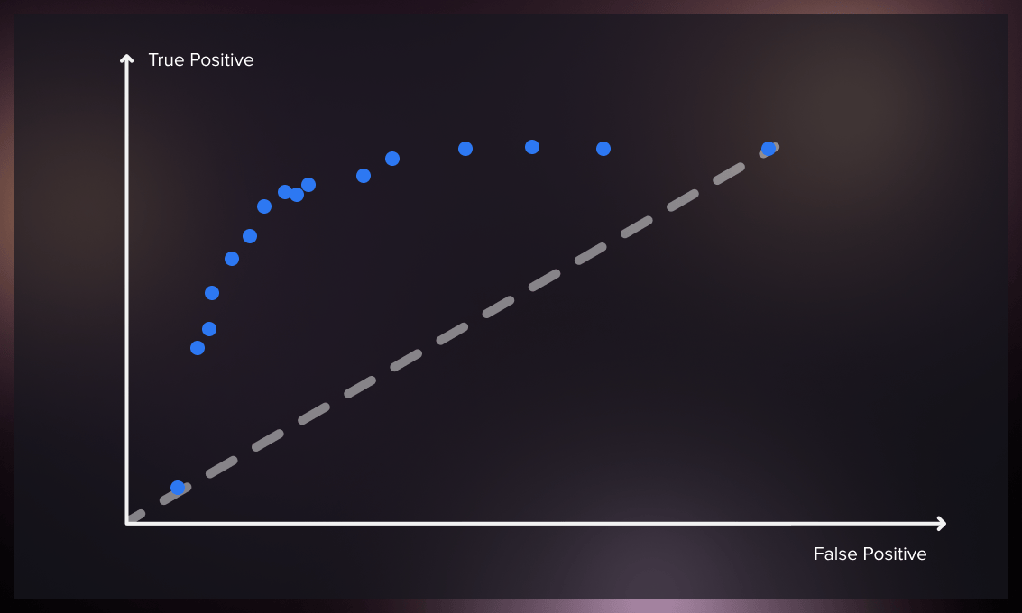
The ROC curve (Receiver Operating Characteristics Curve) is a performance metric used for evaluating classifier models. It illustrates the relationship between the true and false positive rates, providing insights into the classifier’s sensitivity. As the threshold for classification changes, the ROC curve compares the true positive rate and false positive rate.

In an ideal scenario, a classifier would have a ROC curve that reaches a true positive rate of 100% while maintaining zero false positives. The ROC curve enables us to measure the trade-off between the increase in false positives and the number of correctly classified positive instances.

The ROC curve helps select an optimal threshold for a classifier that maximizes true positives and minimizes false positives. It allows us to determine the precise balance between true and false positive rates by using different probability thresholds. It is handy when the dataset contains a balanced distribution of observations across each class. Although initially employed in signal detection, ROC curves have applications in medicine, radiology, natural hazards, and other fields.

A single point on the ROC space is obtained for discrete classifiers that provide only predicted class labels. However, probabilistic classifiers offer probabilities or scores indicating the likelihood of an instance belonging to a particular class. By adjusting the threshold for the score, we can generate a curve that represents the classifier’s performance across various thresholds.

AUC

Area Under Curve (AUC) is a commonly used metric for evaluating models, particularly in binary classification tasks. It quantifies the overall performance of a model by measuring the area beneath the complete ROC curve. AUC represents the likelihood of a randomly selected positive example having a higher ranking than a randomly selected negative example according to the classifier.

AUC serves as a summary measure for the ROC curve and gauges the classifier’s ability to differentiate between classes. A higher AUC value suggests that the model performs better at distinguishing positive and negative instances.

Watch this video for a more detailed explanation of ROC and AUC in machine learning.

In summary, ROC and AUC provide an overall assessment of a classifier’s performance across various thresholds, while F1 score gives a single metric that balances precision and recall. They are complementary evaluation measures that can be used to assess the effectiveness of a ML model.

In addition to ROC and AUC, there are other methods that can be used for evaluating ML models, including the F-beta score, Matthews correlation coefficient, and Jaccard index.

F-beta score

F-beta is an evaluation metric commonly used in machine learning and information retrieval tasks, particularly in the context of binary classification problems. It is an extension of the F1 score, which combines precision and recall into a single measure.

The F-beta score takes into account both precision (the model’s ability to correctly identify positive instances) and recall (the ability of the model to retrieve all positive instances). It allows you to control the balance between precision and recall by adjusting a parameter called beta.

The formula for calculating the F-beta score is as follows:

$$F_{\beta}=(1+\beta^{2})\times \frac{(1+\beta^{2})tp}{(1+\beta^{2})tp + \beta^{2}fn + fp}$$

In this formula, beta determines the weight of recall in the score. A higher beta value emphasizes recall, while a lower beta value gives more weight to precision. When beta is 1, the F-beta score equals the F1 score.

Matthew’s correlation coefficient

Matthew’s Correlation Coefficient (MCC) is a common metric for evaluating the performance of binary classification models. It takes into account:

• true positives (TP)
• true negatives (TN)
• false positives (FP)
• false negatives (FN)

The metric helps achhieve a balanced measure of the classifier’s performance, especially when dealing with imbalanced datasets.

The following formula is used for calculating Matthew’s correlation coefficient:

$$MCC = \frac {TP \times TN - FP \times FN}{\sqrt{(TP + FP)(TP + FN)(TN + FP)(TN + FN)}}$$

MCC ranges from -1 to 1, where 1 represents a perfect prediction, 0 indicates a random prediction, and -1 denotes a total disagreement between the predictions and the true labels.

The MCC metric considers all four elements of the confusion matrix (TP, TN, FP, and FN) and provides a balanced measure of the classifier’s performance.

Jaccard index

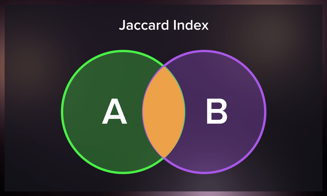
The Jaccard similarity index, or the Jaccard similarity coefficient, compares two sets of members to determine the shared and distinct elements. It is a similarity measure between two datasets, ranging from 0% to 100%. A higher percentage indicates a greater similarity between the populations. However, this metric is sensitive to small sample sizes and can yield misleading results, particularly with limited samples or datasets containing missing observations.

The following formula is used to calculate the Jaccard index:

Jaccard Index = (number of elements in both sets) / (number of elements in either set) * 100

Conclusion

We have covered the essential aspects of the F1 score, including where it is commonly used and how to calculate it. Understanding the F1 score is important because it considers both recall and precision, which is particularly valuable when dealing with imbalanced data – a situation often encountered in real-world scenarios.

However, you need to be aware of the limitations of the F1 score. For example, it doesn’t provide information about the distribution of errors, and it treats precision and recall equally, which may not always be suitable for all situations. Additionally, the F1 score may not capture certain data patterns effectively.

To address these limitations, you should consider your problem’s specific needs and explore alternative evaluation metrics or complementary approaches alongside the F1 score, such as ROC and AUC.

Once it’s done, you can confidently evaluate the performance of your models and make informed decisions.