
In this post, we are going to have a look at the most widely used machine learning algorithms. There is a huge variety of them, and it is easy to feel confused when you hear such terms as “instance-based learning algorithms” and “perceptron”.
Usually, all machine learning algorithms are divided into groups based on either their learning style, function, or the problems they solve. In this post, you will find a classification based on learning style. I will also mention the common tasks that these algorithms help to solve.
The number of machine learning algorithms that are used today is large, and I will not mention 100% of them. However, I would like to provide an overview of the most commonly used ones.
Supervised learning algorithms
If you’re not familiar with such terms as “supervised learning” and “unsupervised learning”, check out our AI vs. ML post where this topic is covered in detail. Now, let’s get familiar with the algorithms.
1. Classification algorithms
Naive Bayes
Bayesian algorithms are a family of probabilistic classifiers used in ML based on applying Bayes’ theorem.
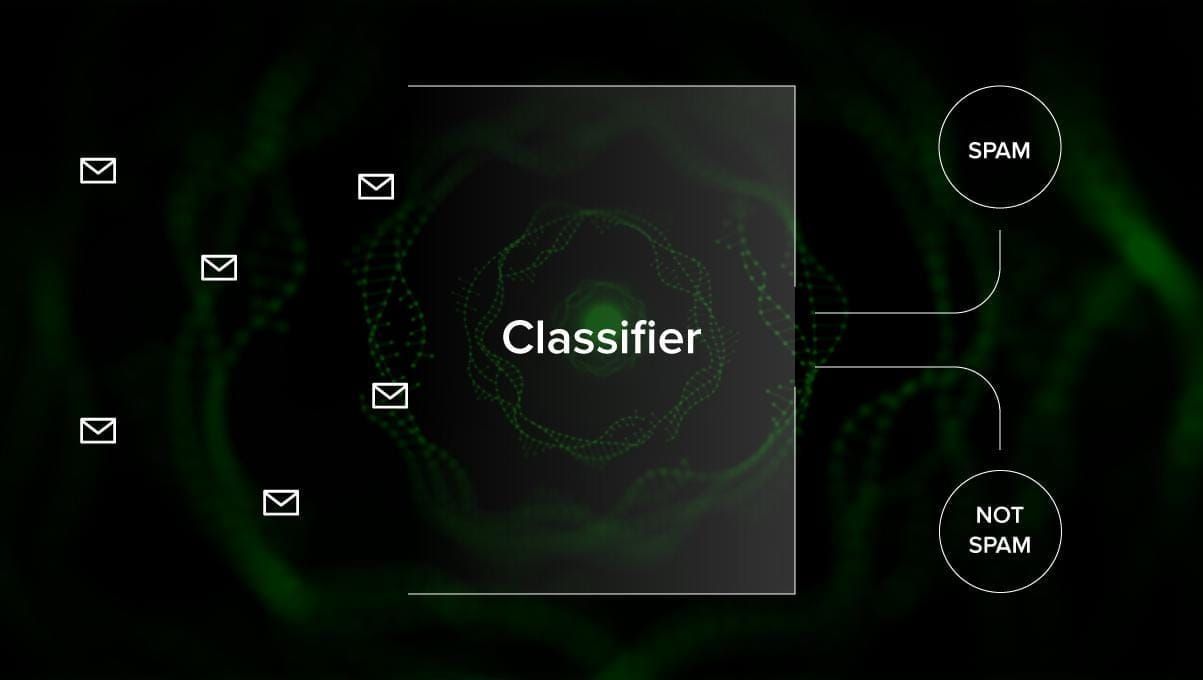
Naive Bayes classifier was one of the first algorithms used for machine learning. It is suitable for binary and multiclass classification and allows for making predictions and forecast data based on historical results. A classic example is spam filtering systems that used Naive Bayes up till 2010 and showed satisfactory results. However, when Bayesian poisoning was invented, programmers started to think of other ways to filter data.
Using Bayes’ theorem, it is possible to tell how the occurrence of an event impacts the probability of another event.
For example, this algorithm calculates the probability that a certain email is or isn’t spam based on the typical words used. Common spam words are “offer”, “order now”, or “additional income”. If the algorithm detects these words, there is a high possibility that the email is spam.
Naive Bayes assumes that the features are independent. Therefore, the algorithm is called naive.
Multinomial Naive Bayes
Apart from Naive Bayes classifier, there are other algorithms in this group. For example, Multinomial Naive Bayes, which is usually applied for document classification based on the frequency of certain words present in the document.
Bayesian algorithms are still used for text categorization and fraud detection. They can also be applied for machine vision (for example, face detection), market segmentation, and bioinformatics.
Logistic regression
Even though the name might seem contra-intuitive, logistic regression is actually a type of classification algorithm.
Logistic regression is a model that makes predictions using a logistic function to find the dependency between the output and input variables. Statquest made a great video where they explain the difference between linear and logistic regression taking as the example obese mice.
Decision trees
A decision tree is a simple way to visualize a decision-making model in the form of a tree. The advantages of decision trees are that they are easy to understand, interpret and visualize. Also, they demand little effort for data preparation.
However, they also have a big disadvantage. The trees can be unstable because of even the smallest variations (variance) in data. It is also possible to create over-complex trees that do not generalize well. This is called overfitting. Bagging, boosting, and regularization help to fight this problem. We are going to talk about them later in the post.
The elements of every decision tree are:
- Root node that asks the main question. It has the arrows pointing down from it but no arrows pointing to it. For example, imagine you are building a tree for deciding what kind of pasta you should have for dinner.
- Branches. A subsection of a tree is called a branch or sometimes a sub-tree.
- Decision nodes. These are the subnodes for the root node that can also be splitting into more nodes. Your decision nodes can be “carbonara?” or “with mushrooms?”.
- Leaves or Terminal nodes. These nodes do not split. They represent final decisions or predictions.
Also, it is important to mention splitting. This is the process of dividing a node into subnodes. For instance, if you’re not a vegetarian, carbonara is okay. But if you are, eat pasta with mushrooms. There is also a process of node removal called pruning.
Decision tree algorithms are referred to as CART (Classification and Regression Trees). Decision trees can work with categorical or numerical data.
- Regression trees are used when the variables have numerical value.
- Classification trees can be applied when the data is categorical (classes).
Decision trees are quite intuitive to understand and use. That is why tree diagrams are commonly applied in a broad range of industries and disciplines. GreyAtom provides a broad overview of different types of decision trees and their practical applications.
SVM (Support Vector Machine)
Support vector machines are another group of algorithms used for classification and, sometimes, regression tasks. SVM is great because it gives quite accurate results with minimum computation power.
The goal of the SVM is to find a hyperplane in an N-dimensional space (where N corresponds with the number of features) that distinctly classifies the data points. The accuracy of the results directly correlates with the hyperplane that we choose. We should find a plane that has the maximum distance between data points of both classes.
This hyperplane is graphically represented as a line that separates one class from another. Data points that fall on different sides of the hyperplane are attributed to different classes.
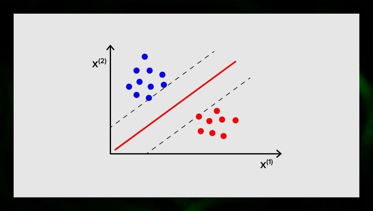
Note that the dimension of the hyperplane depends on the number of features. If the number of input features is 2, then the hyperplane is just a line. If the number of input features is 3, then the hyperplane becomes a two-dimensional plane. It becomes difficult to draw on a graph a model when the number of features exceeds 3. So, in this case, you will be using Kernel types to transform it into a 3-dimensional space.
Why is this called a Support Vector Machine? Support vectors are data points closest to the hyperplane. They directly influence the position and orientation of the hyperplane and allow us to maximize the margin of the classifier. Deleting the support vectors will change the position of the hyperplane. These are the points that help us to build our SVM.
SVM are now actively used in medical diagnosis to find anomalies, in air quality control systems, for financial analysis and predictions on the stock market, and machine fault-control in industry.
2. Regression algorithms
Regression algorithms are useful in analytics, for example, when you are trying to predict the costs for securities or sales for a particular product at a particular time.
Linear regression
Linear regression attempts to model the relationship between variables by fitting a linear equation to the observed data.
There are explanatory and dependent variables. Dependent variables are things that we want to explain or forecast. The explanatory ones, as it follows for the name, explain something. If you want to build linear regression, you assume there is a linear relationship between your dependent and independent variables. For example, there is a correlation between the square metres of a house and its price or the density of population and kebab places in the area.
Once you make that assumption, you next need to figure out the specific linear relationship. You will need to find a linear regression equation for a set of data. The last step is to calculate the residual.
Note: When the regression draws a straight line, it is called linear, when it is a curve – polynomial.
Unsupervised learning algorithms
Now let us talk about algorithms that are able to find hidden patterns in unlabeled data.
1. Clustering
Clustering means that we’re dividing inputs into groups according to the degree of their similarity to each other. Clustering is usually one of the steps to building a more complex algorithm. It is more simple to study each group separately and build a model based on their features, rather than work with everything at once. The same technique is constantly used in marketing and sales to break all potential clients into groups.
Very common clustering algorithms are k-means clustering and k-nearest neighbor.
K-means clustering
K-means clustering divides the set of elements of the vector space into a predefined number of clusters k. An incorrect number of clusters will invalidate the whole process, though, so it’s important to try it with varying numbers of clusters. The main idea of the k-means algorithm is that the data is randomly divided into clusters, and after, the center of each cluster obtained in the previous step is iteratively recalculated. Then, the vectors are divided into clusters again. The algorithm stops when at some point there is no change in clusters after an iteration.
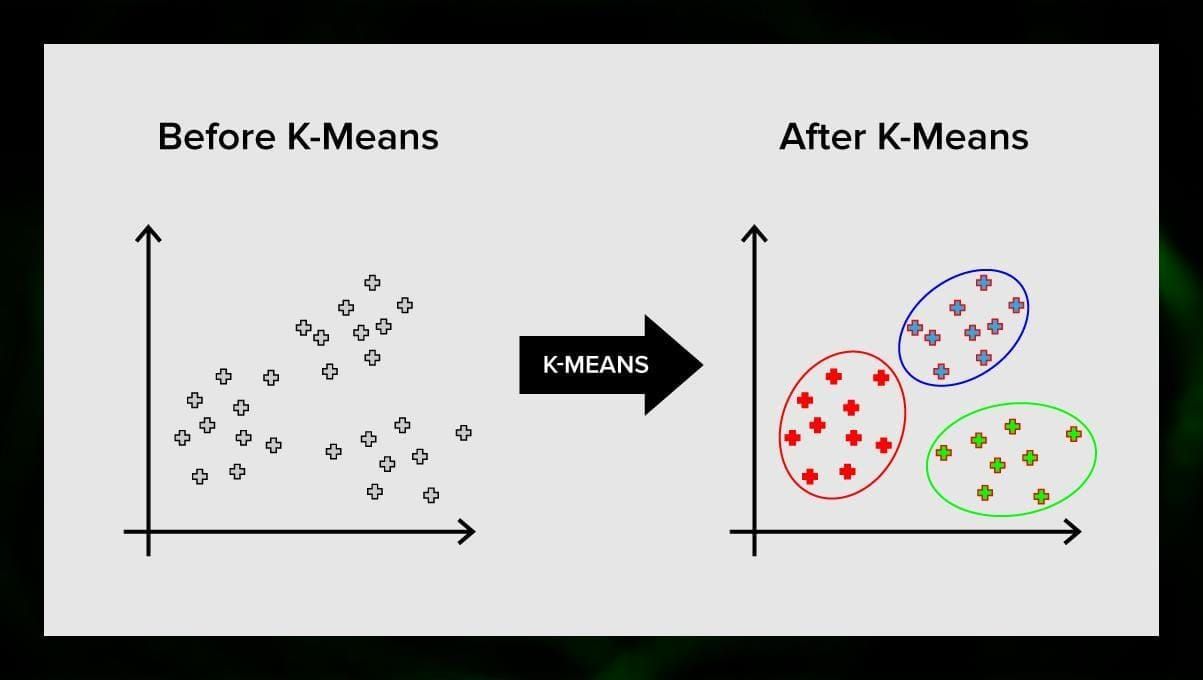
This method can be applied to solve problems when clusters are distinct or can be separated from each other easily, with no overlapping data.
K-nearest neighbor
kNN stands for k-nearest neighbor. This is one of the simplest classification algorithms sometimes used in regression tasks.
To train the classifier, you must have a set of data with predefined classes. The marking is done manually involving specialists in the studied area. Using this algorithm, it is possible to work with multiple classes or clear up the situations where inputs belong to more than one class.
The method is based on the assumption that similar labels correspond to close objects in the attribute vector space.
Modern software systems use kNN for visual pattern recognition, for instance, to scan and detect hidden packages at the bottom of the cart at check-out (for example, AmazonGo). K-nearest neighbor is also used in banking to detect patterns in credit card usage. kNN algorithms analyze all the data and spot unusual patterns that indicate suspicious activity.
2. Dimensionality reduction
Principal component analysis (PCA) is an important technique to understand in order to effectively solve ML-related problems.
Imagine you have a lot of variables to consider. For example, you need to cluster cities into three groups: good for living, bad for living and so-so. How many variables do you have to consider? Probably, a lot. Do you understand the relationships between them? Not really. So how can you take all of the variables you’ve collected and focus on only a few of them that are the most important?
In technical terms, you want to “reduce the dimension of your feature space.” By reducing the dimension of your feature space, you manage to get fewer relationships between variables to consider and you are less likely to overfit your model.
There are many ways to achieve dimensionality reduction, but most of these techniques fall into one of two classes:
- Feature Elimination;
- Feature Extraction.
Feature elimination means that you reduce the number of features by eliminating some of them. The advantages of this method are that it is simple and maintains the interpretability of your variables. As a disadvantage, although, you get zero information from the variables you’ve decided to drop.
Feature extraction avoids this issue. The goal when applying this method is to extract a set of features from the given dataset. Feature Extraction aims to reduce the number of features in a dataset by creating new features based on the existing ones (and then discarding the original features). The new reduced set of features has to be created in a way that it is able to summarize most of the information contained in the original set of features.
Principal component analysis is an algorithm for feature extraction. it combines the input variables in a specific way, and then it is possible to drop the “least important” variables while still retaining the most valuable parts of all of the variables.
One of the possible uses of PCA is when the images in the dataset are too large. A reduced feature representation helps to quickly deal with tasks such as image matching and retrieval.
3. Association rule learning
Apriori is one of the most popular association rule search algorithms. It is able to process large amounts of data in a relatively small period of time.
The thing is that databases of many projects today are very large, reaching gigabytes and terabytes. And they will continue growing. Therefore, one needs an effective, scalable algorithm to find associative rules in a short amount of time. Apriori is one of these algorithms.
In order to be able to apply the algorithm, it is necessary to prepare the data, converting it all to the binary form and changing its data structure.
Usually, you operate this algorithm on a database containing a large number of transactions, for example, on a database that contains information about all the items customers have bought at a supermarket.
Reinforcement learning
Reinforcement learning is one of the methods of machine learning that helps to teach the machine how to interact with a certain environment. In this case, the environment (for example, in a video game) serves as the teacher. It provides feedback to the decisions made by the computer. Based on this reward, the machine learns to take the best course of action. It reminds the way children learn not to touch a hot frying pan – through trial and feeling pain.
Breaking this process down, it involves these simple steps:
- The computer observes the environment;
- Chooses some strategy;
- Acts according to this strategy;
- Receives either a reward or penalty;
- Learns from this experience and refines the strategy;
- Repeats until the optimal strategy is found.
Q-Learning
There are a couple of algorithms that can be used for Reinforcement learning. One of the most common is Q-learning.
Q-learning is a model-free reinforcement learning algorithm. Q-learning is based on the remuneration received from the environment. The agent forms a utility function Q, which subsequently gives it an opportunity to choose a behavior strategy, and take into account the experience of previous interactions with the environment.
One of the advantages of Q-learning is that it is able to compare the expected usefulness of the available actions without forming environmental models.
Ensemble learning
Ensemble learning is the method of solving a problem by building multiple ML models and combining them. Ensemble learning is primarily used to improve the performance of classification, prediction, and function approximation models. Other applications of ensemble learning include checking the decision made by the model, selecting optimal features for building models, incremental learning, and nonstationary learning.
Below are some of the more common ensemble learning algorithms.
Bagging
Bagging stands for bootstrap aggregating. It is one of the earliest ensemble algorithms, with a surprisingly good performance. To guarantee the diversity of classifiers, you use bootstrapped replicas of the training data. That means that different training data subsets are randomly drawn – with replacement – from the training dataset. Each training data subset is used to train a different classifier of the same type. Then, individual classifiers can be combined. To do this, you need to take a simple majority vote of their decisions. The class that was assigned by the majority of classifiers is the ensemble decision.
Boosting
This group of ensemble algorithms is similar to bagging. Boosting also uses a variety of classifiers to resample the data, and then chooses the optimal version by majority voting. In boosting, you iteratively train weak classifiers to assemble them into a strong classifier. When the classifiers are added, they are usually attributed in some weights, which describe the accuracy of their predictions. After a weak classifier is added to the ensemble, the weights are recalculated. Incorrectly classified inputs gain more weight, and correctly classified instances lose weight. Thus, the system focuses more on examples where an erroneous classification was obtained.
Random forest
Random forests or random decision forests are an ensemble learning method for classification, regression, and other tasks. To build a random forest, you need to train a multitude of decision trees on random samples of training data. The output of the random forest is the most frequent result among the individual trees. Random decision forests successfully fight overfitting due the _random _nature of the algorithm.
Stacking
Stacking is an ensemble learning technique that combines multiple classification or regression models via a meta-classifier or a meta-regressor. The base level models are trained based on a complete training set, then the meta-model is trained on the outputs of the base level models as features.
Neural networks
A neural network is a sequence of neurons connected by synapses, which reminds of the structure of the human brain. However, the human brain is even more complex.
What is great about neural networks is that they can be used for basically any task from spam filtering to computer vision. However, they are normally applied for machine translation, anomaly detection and risk management, speech recognition and language generation, face recognition, and more.
A neural network consists of neurons, or nodes. Each of these neurons receives data, processes it, and then transfers it to another neuron.
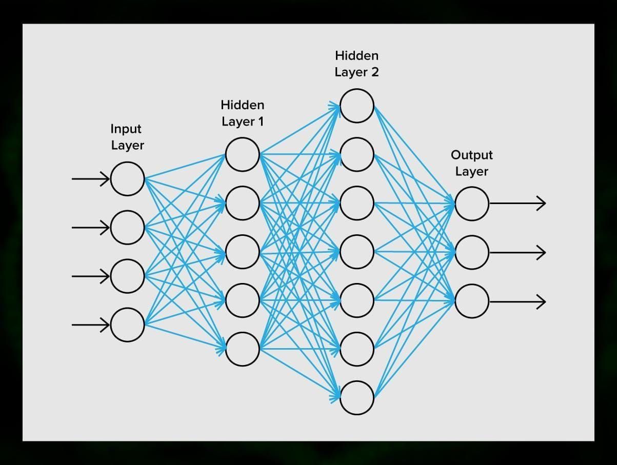
Every neuron processes the signals the same way. But how then do we get a different result? The synapses that connect neurons to each other are responsible for this. Each neuron is able to have many synapses that attenuate or amplify the signal. Also, neurons are able to change their characteristics over time. By choosing the correct synapse parameters, we will be able to get the correct results of the input information conversion at the output.
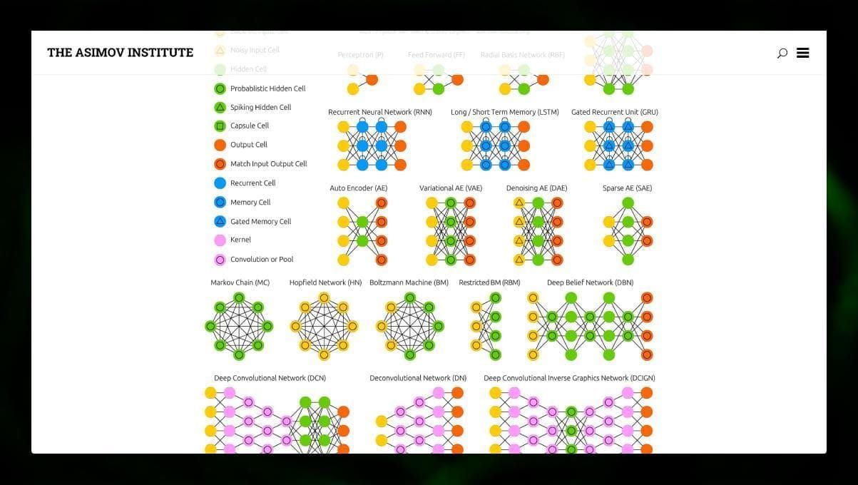
There are many different types of NN:
- Feedforward neural networks (FF or FFNN) and perceptrons (P) are very straightforward, there are no loops or cycles in the network. In practice, such networks are rarely used, but they are often combined with other types to obtain new ones.
- A Hopfield network (HN) is a fully connected neural network with a symmetric matrix of links. Such a network is often called an associative memory network. Just like a person who seeing one half of the table, can imagine the second half, this network, receiving a noisy table, restores it to full.
- Convolutional neural networks (CNN) and deep convolutional neural networks (DCNN) are very different from other types of networks. They are usually used for image processing, audio or video-related tasks. A typical way to apply CNN is to classify images.
Many different types of neural networks are interesting to observe. It is possible to do that in the NN zoo.
Conclusion
This post is a broad overview of different ML algorithms, but there is still a lot to be said. Stay tuned to our Twitter, Facebook, and Medium for more guides and posts about the exciting possibilities of machine learning.
Discover Serokell’s AI consulting services.

.jpg)