Signal Processing in Haskell

Today, I would like to tell you about my work in the laboratory of the Physics Department of Moscow State University, where I study for a Master’s degree.

One of the main activities at our laboratory is research on passing a laser beam through the atmosphere. How can we use it for transferring data? How will it be changed by air fluctuations?

For data transfer, we use a narrow ray (“data beam”). We also send a probing, wide-aperture beam periodically, and by changes in its internal structure (which is really complex) we can recognize the state of the atmosphere along the path. Using that information, we are able to predict distortions of “data beam” and compensate for them by adjusting it.

The main goal of all this is to increase the possible speed of data transferring via an optical beam, which is really low now.

Personally, I develop software for processing the signal coming from a video camera. This signal is generated by a wide-aperture laser beam that passes through a long atmospheric path before reaching the camera lens.

The task of the software is to determine the characteristics of the incoming beam (the moments of the image, up to the 4th), as well as the time-frequency characteristics of these quantities. To determine the frequency components more accurately, we use quadratic time-frequency distributions (QTFD), such as the Wigner-Ville distribution.

One of the important issues is that the time for processing the signal is limited. At the same time, the quadratic time-frequency transforms are nonlocal, which means that to process a certain period of the signal it is necessary to completely obtain all samples from this period, which makes real-time processing impossible.

In this case, it is necessary to strive to have time to process the signal while the samples for the next measurement period are being accumulated, which means that the processing time should not be longer than the duration of the measurement (let’s call it a “quasi-realtime” task). At the same time, this task is easily separable into many threads.

Why Haskell?

In addition to the type safety that minimizes, to a certain extent, the number of errors at runtime, Haskell makes it easy and quick to parallelize the calculations. Furthermore, there’s a Haskell library called Accelerate that makes it easy and convenient to use the resources of the GPU.

An important drawback of Haskell for latency-sensitive tasks is the garbage collector, which periodically completely stops the program. This is partially offset by the fact that there are tools to minimize the delays associated with it, in particular - the use of “compact regions”. With it you are able to specify to the garbage collector that a certain set of data should not be deleted while at least one element of the set is used. This allows you to significantly reduce the time spent by the garbage collector to check the data set.

In addition, the laziness of the language proves to be advantageous. This may seem strange: laziness often provokes criticism because of the problems it creates (memory leaks due to uncalculated thunks), but in this case, it is beneficial due to the possibility of dividing the description of the algorithm and its execution. This helps to ease the parallelization of the task, because often there is almost no need to make any changes to the already prepared algorithm, because after describing the calculations, we did not prescribe how or when they should be performed. In case of imperative languages, scheduling computations falls entirely on the shoulders of the programmer - they determine when and what actions will be performed. In Haskell, this is done by the runtime system, but we can easily specify what should be done and how.

The first task: obtaining the moments of images from a video recording of a laser beam

In this task, the ffmpeg-light and JuicyPixels libraries were used for data processing.

The task can be decomposed into several steps: obtaining images, determining the moments of the image, and obtaining statistics on these moments throughout the video file.

data Moment =
      ZeroM   { m00 :: {-# UNPACK #-}!Int }
    | FirstM  { m10 :: {-# UNPACK #-}!Int,    m01 :: {-# UNPACK #-}!Int }
    | SecondM { m20 :: {-# UNPACK #-}!Double, m02 :: {-# UNPACK #-}!Double
              , m11 :: {-# UNPACK #-}!Double }
    | ThirdM  { m30 :: {-# UNPACK #-}!Double, m21 :: {-# UNPACK #-}!Double
              , m12 :: {-# UNPACK #-}!Double, m03 :: {-# UNPACK #-}!Double }
    | FourthM { m40 :: {-# UNPACK #-}!Double, m31 :: {-# UNPACK #-}!Double
              , m22 :: {-# UNPACK #-}!Double, m13 :: {-# UNPACK #-}!Double
              , m04 :: {-# UNPACK #-}!Double }

The video image was converted to a list of images of Image Pixel8 type that were collapsed using the appropriate functions. Parallel processing is performed as follows:

processFrames :: PixelF -> PixelF -> [Image Pixel8] ->  V.Vector TempData
processFrames cutoff factor imgs = 
    foldl' (\acc frameData -> (acc V.++ frameData)) (V.empty) tempdata
    where tempdata = P.parMap P.rdeepseq (processFrame cutoff factor) imgs

This function takes 2 auxiliary parameters (background value and scaling factor), a list of images and returns a vector of values of type TempData (it stores moments and some other values, which will later be analyzed statistically).

Processing each image is done in parallel, using the parMap function. The tasks are resource-intensive, so the costs of creating separate threads pay off.

Example from another program:

sumsFrames :: (V.Vector (Image Pixel8), Params) -> V.Vector (V.Vector Double, V.Vector Double)
sumsFrames (imgs, params) = 
    (V.map (sumsFrame params) imgs) `VS.using` (VS.parVector 4)

In this case, the result of the calculation is started using the using function:

using :: a -> Strategy a -> a

which starts the computation of a given value of type a using the appropriate strategy, in this case - 4 elements per thread, because the calculation of one element is too quick and the creation of a separate thread for each element would cause a high overhead.

As you can see from the previous examples, parallel execution almost does not change the code itself: in the second example, you can just remove VS.using (VS.parVector 4) and the final result will not change at all, calculations will simply take longer.

The second task: time-frequency analysis of the obtained values

After processing the video recording with laser beam oscillations, we get a set of values, for some of which it is necessary to build a time-frequency distribution. A common method is spectrogram construction, but it gives a relatively low resolution — and the higher we make it in frequency, the worse it will be in time and vice versa. You can work around this restriction by using Cohen class transforms:

$$C_x(t, \omega;f) = \iiint_{-\infty} e^{-i\phi(s-t)} f(\phi,\tau) x(s+\tau/2)x^{*}(s-\tau/2) e^{-i\omega\tau}d{\phi}dsd{\tau}$$

Here x (t) is the initial signal and f (φ, τ) is the parameterization function, by means of which a specific transformation is specified. The simplest example is the Wigner-Ville transform:

$$WV (t,\omega) = 2 \int_{-\infty}^{\infty}x(t+n)x^{*}(t-n)e^{-2i{\omega}n}dn$$

A comparison of the spectrogram and the Wigner-Ville distribution is given below.

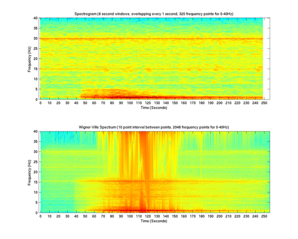
The second graph is more detailed (especially in the low-frequency region), but there are interference components in it. To combat them, various anti-aliasing methods or other transformations of the Cohen class are used. The calculation takes place in several stages:

1. Perform the Hilbert transformation (we obtain an analytical signal)
2. Construct the matrix A = x (t + n)* x (t-n)
3. Apply a 1D Fourier transform to every column of the matrix

An example of an algorithm for calculating a more complex transformation of the Cohen class (Choi-Williams) can be found here.

To calculate these transformations, the Accelerate library was used. This library makes it possible to use both the central processor (with effective distribution of the load on the cores) and the graphics processor at the request of the user (even without rebuilding the program).

The library uses its own DSL, which is compiled into LLVM code at runtime, which can then be compiled into both the code for the CPU and the code for the GPU (CUDA). The computational cores formed for the graphics processor are efficiently cached, preventing recompilation in runtime unnecessarily. Thus, when one performs a large number of the same tasks, the code compilation in runtime occurs only once.

The DSL of Accelerate is similar to the DSL of REPA (Regular Parallel Arrays library) and rather intuitive, the values ​​of the type Acc a are in reality code that is generated in the compile-time (That is why, when trying to output to GHCi a value of the type, for example, Acc (Array DIM1 Int), it will output not an array of integers but some code to calculate it). This code is compiled and run by separate functions, such as:

run :: Arrays a => Acc a -> a

or

runN :: Afunction f => f -> AfunctionR f

These functions compile the code (written in acelerate’s DSL) with applying various optimizations, such as fusion.

In addition, the latest version has the ability to run the compilation of expressions (using the runQ function) at Haskell compile time.

Example of the Wigner-Willy transformation calculation function:

...
import Data.Array.Accelerate as A
import qualified Data.Array.Accelerate.Math.FFT as AMF
...
-- | Wigner-ville distribution. 
-- It takes 1D array of complex floating numbers and returns 2D array of real numbers.  
-- Columns of result array represents time and rows — frequency. Frequency range is from 0 to n/4,  
-- where n is a sampling frequency.  

wignerVille 
  :: (A.RealFloat e, A.IsFloating e, A.FromIntegral Int e, Elt e, Elt (ADC.Complex e), AMF.Numeric  e)  
  => Acc (Array DIM1 (ADC.Complex e))  -- ^ Data array  
  -> Acc (Array DIM2 e)  
wignerVille arr =  
  let times = A.enumFromN (A.index1 leng) 0 :: Acc (Array DIM1 Int)
      leng = A.length arr 
      taumx = taumaxs times
      lims = limits taumx
  in A.map ADC.real $ A.transpose $ AMF.fft AMF.Forward $ createMatrix arr taumx lims 

Thus, we are able to use the resources of the GPU without a detailed study of CUDA, and we obtain type safety that helps us cut off a large number of potential errors.

After that, the resulting matrix is loaded from the video memory into RAM for further processing.

In this case, even on a relatively weak video card (NVidia GT-510) with passive cooling, calculations take place 1.5-2 times faster than on a CPU. In our case, the Wigner-Willy transformation for 10,000 points occurs faster than in 30 seconds, which fits perfectly into the notion of quasi-realtime (and this value can be much smaller on more powerful GPUs). Based on this information, the original laser beam will be corrected to compensate for atmospheric pulsations.

In addition, results of this time-frequency distributions are permanently saved to disk in text form for later analysis. Here I was faced with the fact that the double-conversion library converts numbers directly to Text or Bytestring, which creates a large load in the case of huge data sets (10 million values or more), so I wrote a patch that adds conversion to Builder values (for Bytestring and Text), and this accelerated the speed of storing text data by 10 times.

In the case of a large number of small pieces of data, they are moved to the compact region if it is possible. This increases memory consumption, but significantly reduces delays associated with the operation of the garbage collector. In addition, the garbage collector is usually started in a single thread, because the parallel garbage collector often introduces large delays.

Conclusion

Methods of accurate time-frequency analysis are very useful in many areas, like medicine (EEG analysis), geology (where non-linear time-frequency analysis is used for a long time), acoustic signal processing. I even found an article (and it was really useful) about using quadratic time-frequency distribution to analyze the vibrations of an engine.

Problem of time-frequency distribution has not been solved for now, and all methods have their own advantages and disadvantages. Fourier transform (STFT) with sliding window shows you real amplitudes, but has a low resolution, Wigner-Ville distribution has an excellent resolution, but it shows only quasi-amplitude - value, that can show where the amplitude is higher and where is lower and has high level of interference cross-term. Many QTFDs are trying both to combat the interferences and not lose resolution (a difficult task).

Regarding the Accelerate library, I can say that it was hard at the beginning to avoid nested parallelism, which is not allowed (and unfortunately is not detected at compile time).

I published the first version of this software as window-ville-accelerate package. Now I’ve added Choi-Williams and Born-Jordan distributions. In the future, I want to add some more distributions and publish it as qtfd-accelerate package.