Training machine learning models requires a lot of data, which is not always available. This is where transfer learning comes into play as it leverages previously trained models. In this blog post, we’ll explore the definition, methodology, benefits, and applications of transfer learning. We’ll also discuss various transfer learning strategies and provide a selection of pre-trained models.
What is transfer learning?
Transfer learning is an ML method that uses a pre-trained model as the basis for training a new one. For example, a model trained for facial recognition can be adjusted for MRI scan analysis. Whereas it’s hard to collect and label thousands of similar images with cancer to train the model from scratch, fine-tuning a ready model is much easier.
The idea is simple: since the machine learning model already knows how to classify a certain type of pictures, it can learn to recognize images with particular diseases, such as traumatic brain injury or cancer metastasis. Through transfer learning, we can achieve very accurate results faster.
The same is true for natural language processing tasks. Thus, if a model has been trained for the sentiment analysis of English-language texts, it can be used for building a model for the same tasks in German or Spanish.
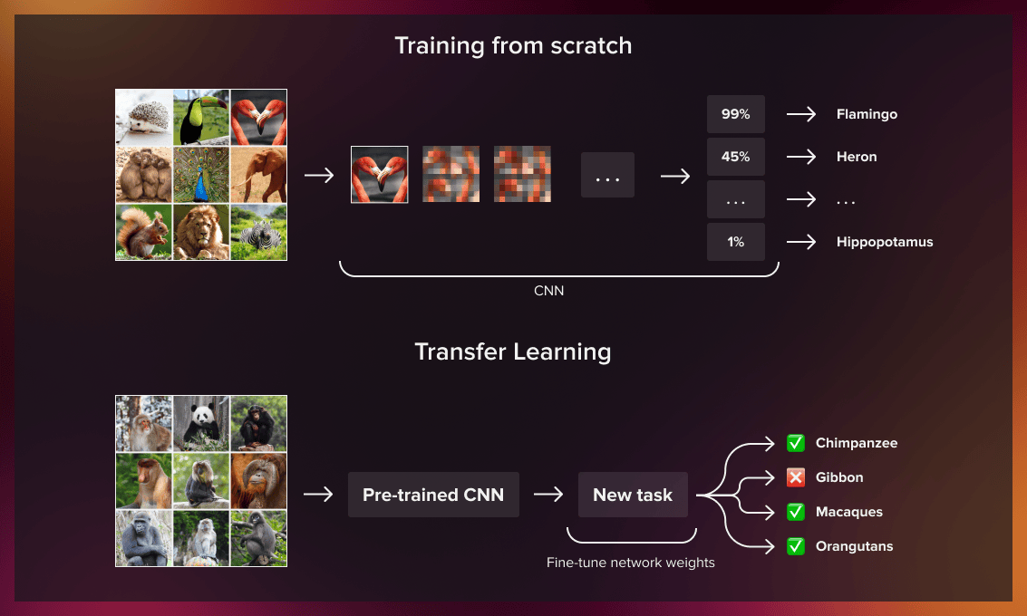
How does transfer learning work?
As the first step in developing your transfer learning strategy, you need to answer the following questions:
- What knowledge can be transferred from the source to the target model to improve the execution of the target task?
- How can we apply the knowledge we learned from the source model to our current project/domain?
- How to avoid model overfitting?
We’ll look at all these issues below.
Three categories of transfer learning
Depending on the task and the amount of labeled/unlabeled data available for source and target domains, transfer learning methods fall into one of three categories: inductive, transductive, and unsupervised.
| Category | Source data labeled? | Target data labeled? |
| Inductive | Can be labeled and unlabeled | Yes |
| Transductive | Yes | No |
| Unsupervised | No | No |
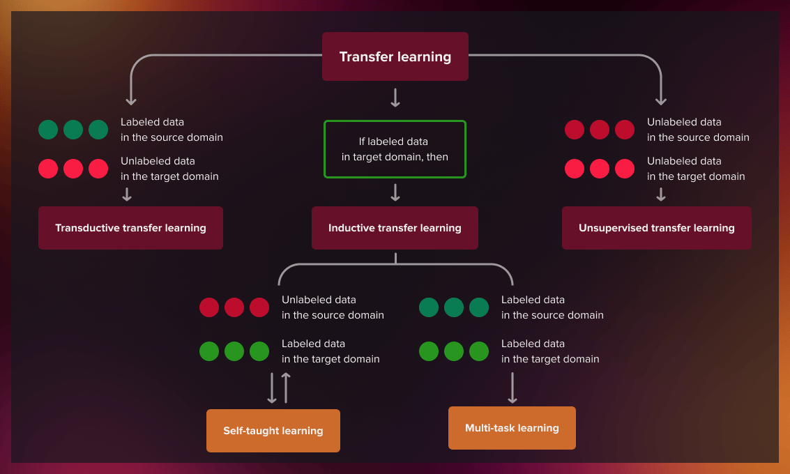
We use different transfer learning approaches depending on the accessibility of data.
Inductive transfer learning
Inductive transfer learning is used when labeled data is the same for the target and source domain but the tasks the model works on are different. The difference between the two domains is in data distribution and label definition. Here, the model encounters training data during the learning process and applies the learned knowledge to improve its performance with a new dataset that may be thematically very similar to the source database (for example, it can recognize tracks based on the model that is trained to identify vehicles).
The source and the target models can be trained successively, in which case the process is called representational transfer. We can use literal transfer (the source model is not modified) or non-literal transfer (the model is altered before transferring knowledge to the target model).
Let’s examine the text classification problem to see how inductive learning (representational transfer) works in practice.
For many years, various text classification models have been trained worldwide. We can combine the results of several of them and develop our own models, which can achieve better quality in classifying text. This is precisely how Google’s algorithm for detecting spam in text works.
To better understand the details, read about the “meta-learn” transfer learning process here.
Another way is to teach the target model concurrently. In this case, depending on whether the source domain contains or lacks labeled data, inductive transfer learning is divided into two subcategories:
-
Multi-task learning: an ML approach in which we teach a shared model multiple tasks simultaneously, based on the labeled source and target domain data.
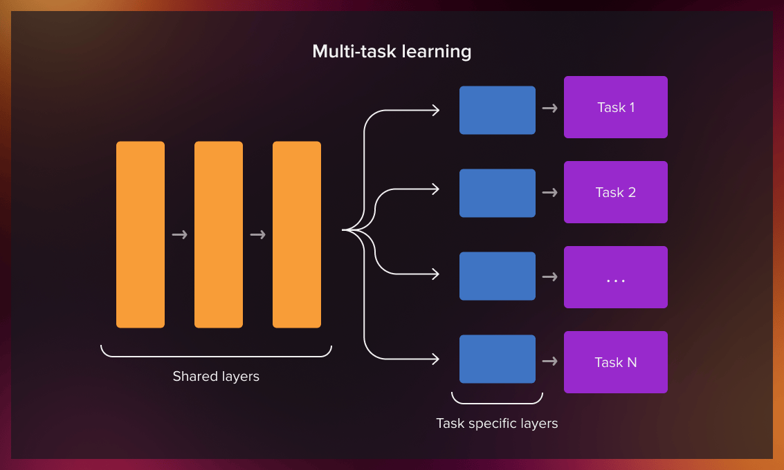 (This approach is widely used in pharmaceutical research, where different drugs are assigned to groups of volunteers whose diagnosis is known. This allows us to evaluate the efficiency of the treatment.)
 -
Self-taught learning: a framework that uses unlabelled data for supervised self-learning. We can transfer the learned pattern to the labeled target domain.
To illustrate this practice, let’s consider how to recognize bicycles in traffic.
We assume that a set of data (vehicle images) can be easily collected from the Internet. This collection is unlabelled and we can teach the model to recognize and categorize cars/trucks/bikes. In self-taught learning, the neural network decides for itself which similarities individual transport objects have and which of their features are important.
Now we can give the model a limited number of bicycles. The recognition accuracy of bicycles using the self-supervised transfer learning will be higher in comparison to the work of the initial model.
Transductive transfer learning
The transductive transfer learning approach is used in scenarios where the domains of the source and target tasks are similar but not exactly the same. In these cases, the source domain usually has a large amount of labeled data, and the target domain contains only a limited amount of unlabeled data.
As a practical example of transductive learning, let’s consider reconstructing different emotions for specific individuals for whom we have a limited number of photographs.
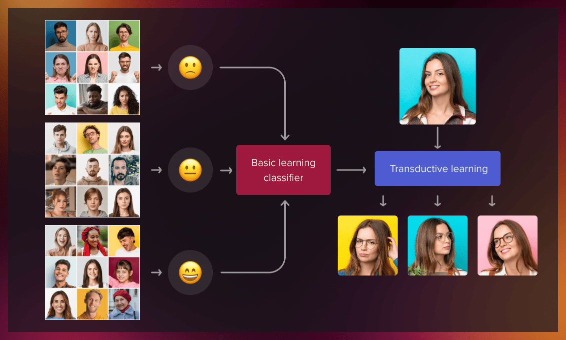
If we have a large database of people’s reactions, we can take a pre-trained model and transfer the knowledge to teach the model to reconstruct the facial expression for that particular person.
In transductive learning, the model has observed both the training and testing datasets before. We predict the labels of the testing dataset by learning from the familiar dataset. We might not know the labels of the testing one but still use its patterns in the learning process.
Unsupervised transfer learning
It works similarly to inductive transfer learning. The difference is that the algorithms focus on unsupervised tasks for both source and target tasks.
So here we are talking about the most common situation where labeled data is not available for both the source and the target domain. This involves a variety of use cases, the most popular of which is anomaly detection.
Whenever labeling data is time-consuming, labor-intensive, or even impossible, unsupervised transfer learning is the only option.
A real-world example is multispectral pedestrian detection. The error cost for driverless cars misdetecting pedestrians is human life. To train the model, we need to provide many cases with different weather conditions, landscapes, people, additional objects that partially obscure the pedestrians. The most complicated part of this task is identifying children.
In real life, it’s almost impossible to have all this data available for all the different scenarios and their combinations. In this situation, transfer learning would be the only option. We can obtain the best result by using self-supervised learning as a basic domain for adults and transfer learning for improving the accuracy of children detection. Check out a detailed review of this case here.
Step-by-step plan for the transfer learning process
The transfer learning process consists of the following steps.
- Create a base model and load pre-trained weights into it.
- Freeze all layers in the base model. (This means that the parameters within the original layers of the model will not change to avoid the possible loss in generalization. We only modify the parameters of the output layer.)
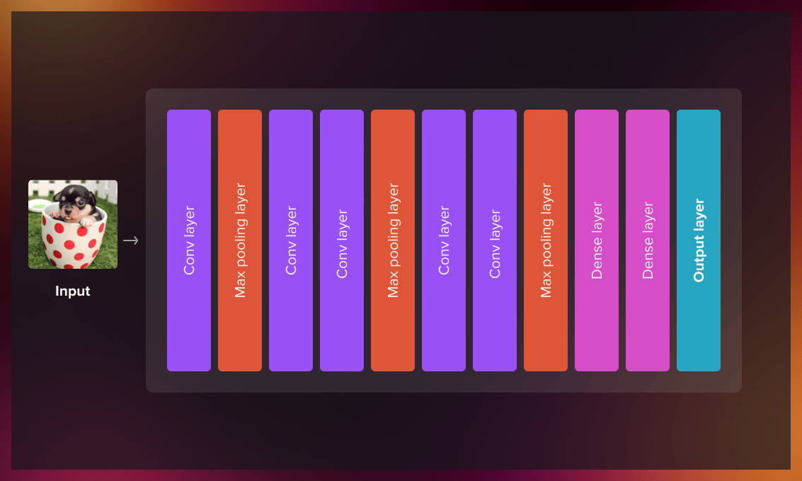
- Create a new model on top of one or several lower-level layers of the base model.
- Train your new model on the new dataset.
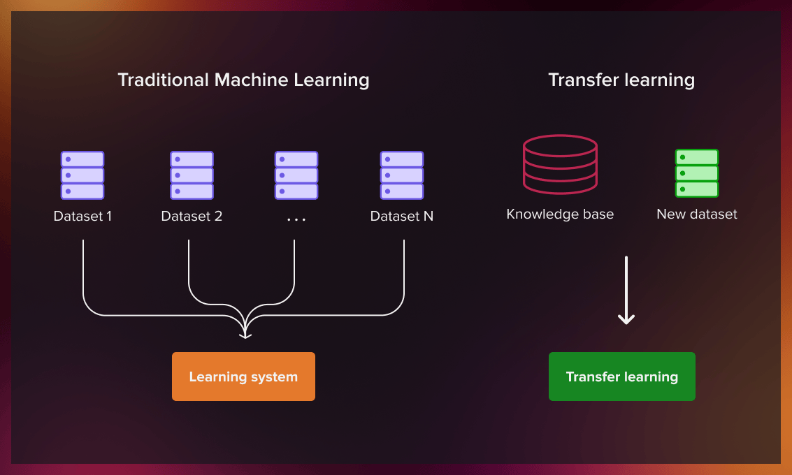
What’s the difference between traditional machine learning and transfer learning?
Transfer learning aims to overcome some limitations and challenges of traditional machine learning models. The table below shows the differences between the two approaches.
| Traditional ML model | Transfer learning model | |
| Amount of data | Requires a large amount of data | Can use a small dataset |
| Costs | Computationally expensive | Cost-effective due to less computation |
| Training | Each model is trained independently for a particular task | The model uses knowledge obtained from the pre-trained model |
| Time | Takes a long time to teach the model | Achieves results faster because transfer learning algorithms leverage features and weights from previously trained models |
Transfer learning strategies
Reusing a model
Imagine you are trying to identify Parkinson disease in the initial stages, but cannot train a deep neural network due to insufficient data. One way around this is to find a task that detects the same disease in the later stages and has a large amount of data. The deep neural network is trained on the second task and then applies its knowledge to the new task.
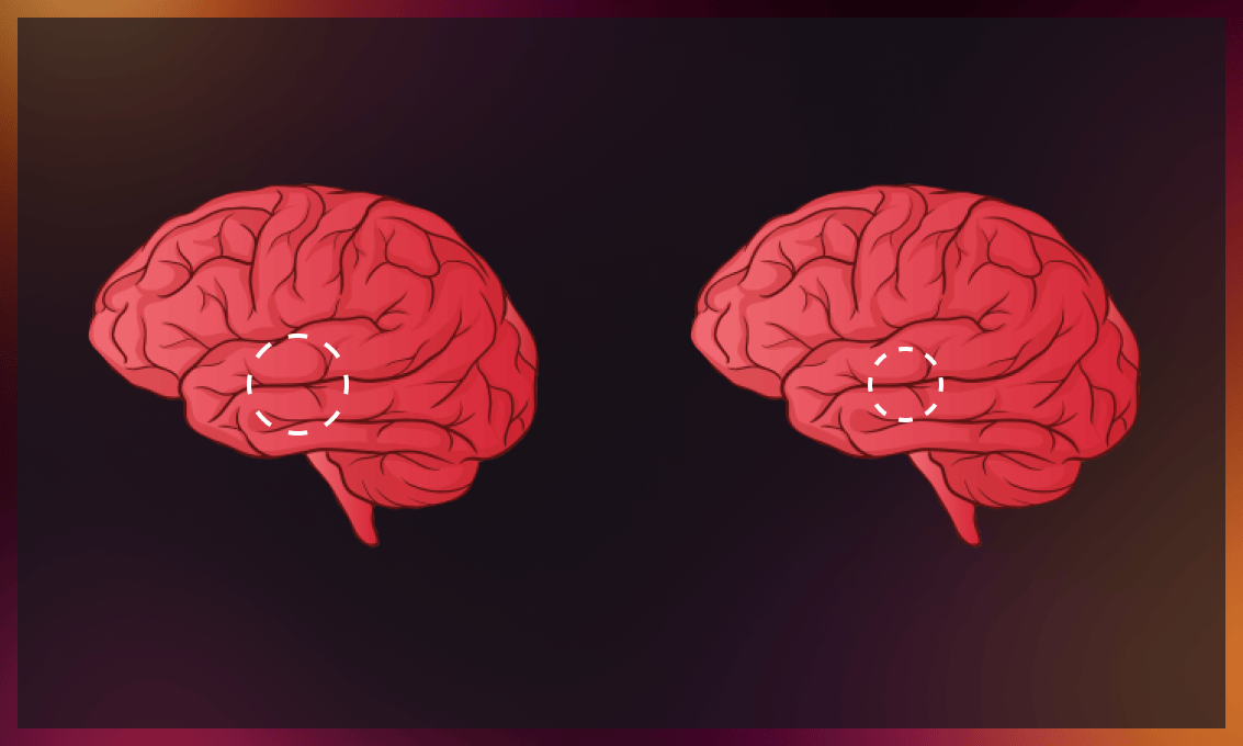
Whether you need to use the entire model or just a few layers depends on the problem you want to solve.
If your inputs are the same for both tasks, you may be able to reuse the model and make predictions for the new inputs. An alternative strategy is to change and re-train the output layer and some task-specific layers.
Using a pre-trained model
The second strategy is using a model that has already been trained. There can be several such models, so make sure you do some research. The number of new trainable layers and the number of reused layers will depend on the problem at hand.
For example, Keras, Model Zoo, and TensorFlow offer pre-trained models that can be used for feature extraction, transfer learning, prediction, and fine-tuning. You will find a list of useful resources at the end of this post.
Feature extraction
Initially, researchers manually hand-craft the features used in machine learning. Deep learning nets can extract features automatically. However, you still have to choose which features to include in your network, which means feature engineering and expertise are still essential. Nevertheless, neural networks can learn which features are important and which are not with the help of a representation learning algorithm. It can quickly identify a desirable combination of features, even for complex tasks that require a lot of human work.
The learned representation can then be applied to other tasks. For that, you should use the first layers to determine the correct representation of features. You simply feed data into your network and use the output layer as an intermediate layer. This intermediate layer will then represent raw data.
Watch this video to learn more about the implementation of transfer learning in practice.
When to use transfer learning?
ML practitioners can apply transfer learning in the following situations:
Insufficient data
Working with little data would result in poor performance. The use of a pre-trained model helps create more accurate models.
Lack of time
Teaching some machine learning models takes too long. Use a similar, pre-trained model when you don’t have enough time to build a new one.
Limited computation capabilities
Too many machine learning tasks needed to train the model require a lot of computation, so the introduction of the pre-trained model is a great help.
When not to use transfer learning?
Insufficient features
Transfer learning is not effective if the features learned by the lower layer (the classification layer) are not sufficient to distinguish the classes for a new problem. If you are trying to understand if transfer learning is applicable in your case, think of the classic “dogs and cats” example. Suppose we have classified the former and now want to identify the latter. In this situation, low-level feature representations are still valid, mid-level are partially valid and high-level ones are invalid in this case. So you can use the low-level features of the pre-trained model instead of the high-level features. In addition, you will need to retrain more layers or, in the worst case, retrain the model from scratch if even deeper layers don’t provide sufficient results.
Unrelated datasets
The features transfer poorly if the datasets are not similar. This would require restricting the parameters that can be trained and removing some layers, which can lead to overfitting. It’s very hard and time-consuming to determine how many layers can be removed without overfitting.
Larger datasets
Transfer learning may not have the expected effect on tasks that require larger datasets. The process of traditional machine learning involves tuning randomized weights until they converge. Transfer learning starts with a pre-trained model, but larger data sets also lead to more iterations, so your initial weights become irrelevant.
Developers cannot eliminate the network layers in transfer learning to confidently identify the best AI models. Dense layers are affected when you remove the first layers because the number of trainable parameters changes. Dense layers can also be a helpful starting point for layer reduction, but determining how many layers and neurons to keep to prevent model overfitting takes a lot of time and effort. Overfitting occurs when a new model picks up unnecessary data and noise from the training data that affects its results.
Read this paper to learn more about the impact of the dataset size on transfer learning.
Benefits of transfer learning
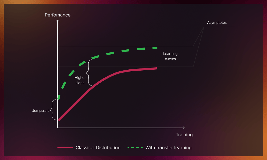
Better initial model
In other learning approaches, you need to build a model that has no prior knowledge. Transfer learning provides a better starting point for performing tasks.
Higher learning rate
Since the model has already been trained on a similar task, transfer learning provides a higher learning rate.
Higher accuracy after training
Transfer learning allows a machine learning model to produce more accurate results thanks to a better baseline and a higher learning rate.
Faster training
Learning using a pre-trained model can achieve target performance faster than traditional machine learning approaches.
Transfer learning vs. fine-tuning
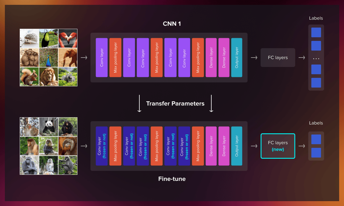
Fine-tuning is a technique of transfer learning where you change the model output to fit a new task. Now let’s look at the difference between transfer learning and fine-tuning.
Transfer learning is the process by which we apply a model created for one task to another. We train the model using a dataset. The same model is then trained with a second dataset with a different class distribution (or even with classes not present in the first training dataset).
Fine-tuning is a particular approach to transfer learning, where we train only the output model and adjust the model to the new task. First, we use around 90% of the dataset for training and then proceed with the remaining 10% for the same model. Usually, we reduce the learning rate so that it has little effect on the weights that have already been changed.
You can also use a base model that is currently performing a similar task and then freeze parts of the layers to preserve the previously learned knowledge when you conduct a training with new data. The training output layer can also be different and some parts of it frozen.
Applications of transfer learning
Image recognition
Transfer learning can be applied to a variety of image recognition applications. For example, a model trained to recognize horses can be further applied to detect zebras.
Natural language processing
One of the best-known applications of transfer learning is natural language processing (NLP). For instance, models that can understand linguistic structures can be used for more complicated tasks such as recommending the next word in a sequence based on previous sentences.
Speech recognition
An ML model designed for Italian speech recognition can be used as the foundation for a Spanish speech recognition model.
Medical imaging
A model developed for analyzing MRI scans can be the basis for a model trained to read CT scans.
Autonomous driving
In autonomous driving, a model developed for recognizing cars on the road, can learn to identify motorcyclists.
Pre-trained models for transfer learning
Here’s a list of popular computer vision models:
ResNet-50
ResNet-50 is a pre-trained convolutional neural network containing 50 layers. Its pre-trained version contains more than a million images from ImageNet. ResNet-50 can classify images into 1000 categories with 92.1% accuracy.
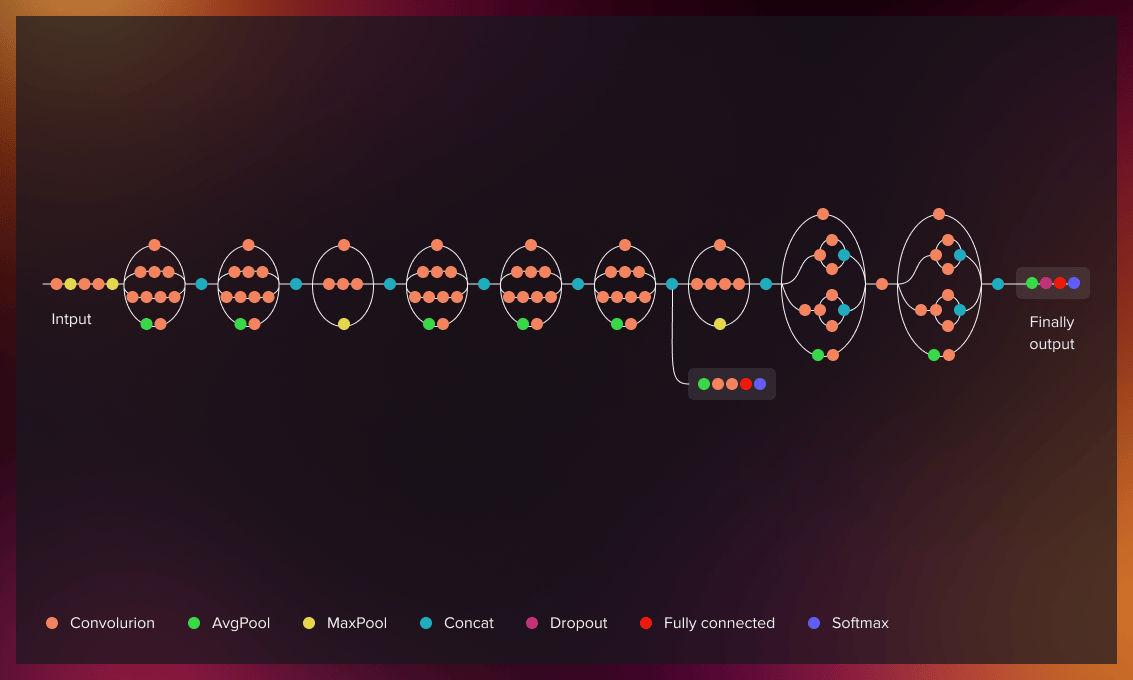
Inception V3
Inception V3 is an image recognition model with more than 78.1% accuracy. It started as a module for Googlenet and was originally introduced as part of the ImageNet Recognition Challenge.
XCeption
Xception is inspired by the Inception model. It contains 71 depthwise separable convolutional layers. It has 94.5% accuracy.
VGG-16
VGG16 is one of the most popular algorithms for object detection and classification from the Kaggle platform. It classifies images from 1000 categories with 92.7% accuracy.
VGG-19
The VGG-19 convolutional network is 19 layers deep. It has feature representations for 1000 categories (a variety of animals and objects such as a pencil, keyboard, mouse, etc.) and can classify images with 90% accuracy.
The following models are helpful for NLP tasks:
Word2Vec
Word2vec is a two-layer NN that turns text into a numerical form (vectors) for further processing by deep neural networks. It is used for discerning patterns in code, genes, social media graphs, etc. Its accuracy is 92.5%.
FastText
FastText is a library for word embedding and text classification learning. The mode, developed by Facebook’s AI research team, enables the development of supervised and unsupervised learning algorithms for word vector representations. Facebook offers pre-trained models in 294 different languages. The accuracy of fastText varies depending on semantic and syntactic categories.
GloVe
GloVe is an unsupervised learning model for creating vector representations. Training is performed using corpus-based global word-word co-occurrence statistics. It has 75% accuracy.
More resources
Microsoft also offers several pre-trained models with the MicrosoftML R and Microsoftml Python packages, both available for development in R and Python.
Model Zoo is a platform with a collection of various pre-trained models for deep learning researchers.
You will find more pre-trained machine learning models in this post.
As an AI and ML company, Serokell provides customized services for your specific purposes. Reach out to us to learn about the solutions we offer.


.jpg)

.jpg)
.jpg)
.jpg)
.jpg)