The support vector machine (SVM) algorithm is a machine learning algorithm widely used because of its high performance, flexibility, and efficiency. In most cases, you can use it on terabytes of data, and it will still be much faster and cheaper than working with deep neural networks.
The algorithm is used for a wide range of tasks such as text classification, handwriting and face recognition, and identification of genes, among others.
In some cases, support vector machines enable simplified application of other ML methods. For example, you can combine CNN and SVM, as described here.
What is a support vector machine?
A support vector machine (SVM) is a supervised ML algorithm that performs classification or regression tasks by constructing a divider that separates data in two categories. The optimal divider is the one which is in equal distance from the boundaries of each group.
The algorithm is more commonly used for classification than regression. In some articles, the SVM for regression is also called support vector regression (SVR). Check out this post to learn more about SVR.
How does the support vector machine classifier work?
As a starting point, let’s consider a simple example with a two-dimensional dataset.
Suppose we have a dataset with two features – x and y – where each entry is tagged with one of two classes (represented with yellow and green colors). Our goal is to build a classifier that can classify unknown points into one of these classes according to their features.
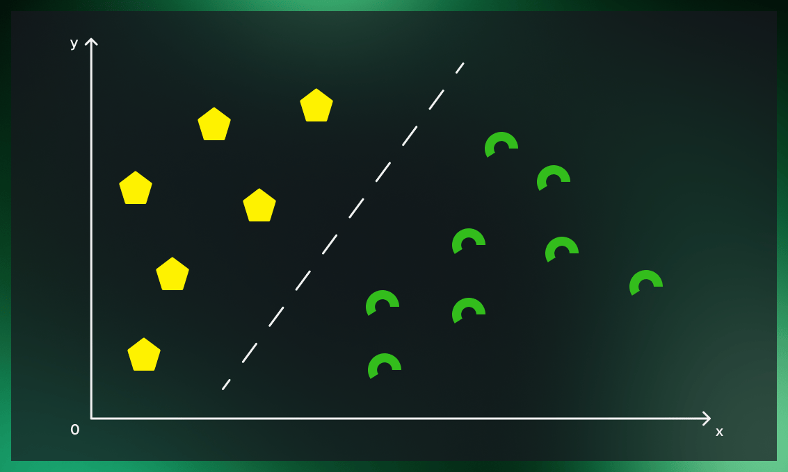
The obvious way of dividing these classes would be to draw a line that separates the entries with “yellow” and “green” classes. But there is an infinite number of possible lines to draw. How can we know which one is correct?
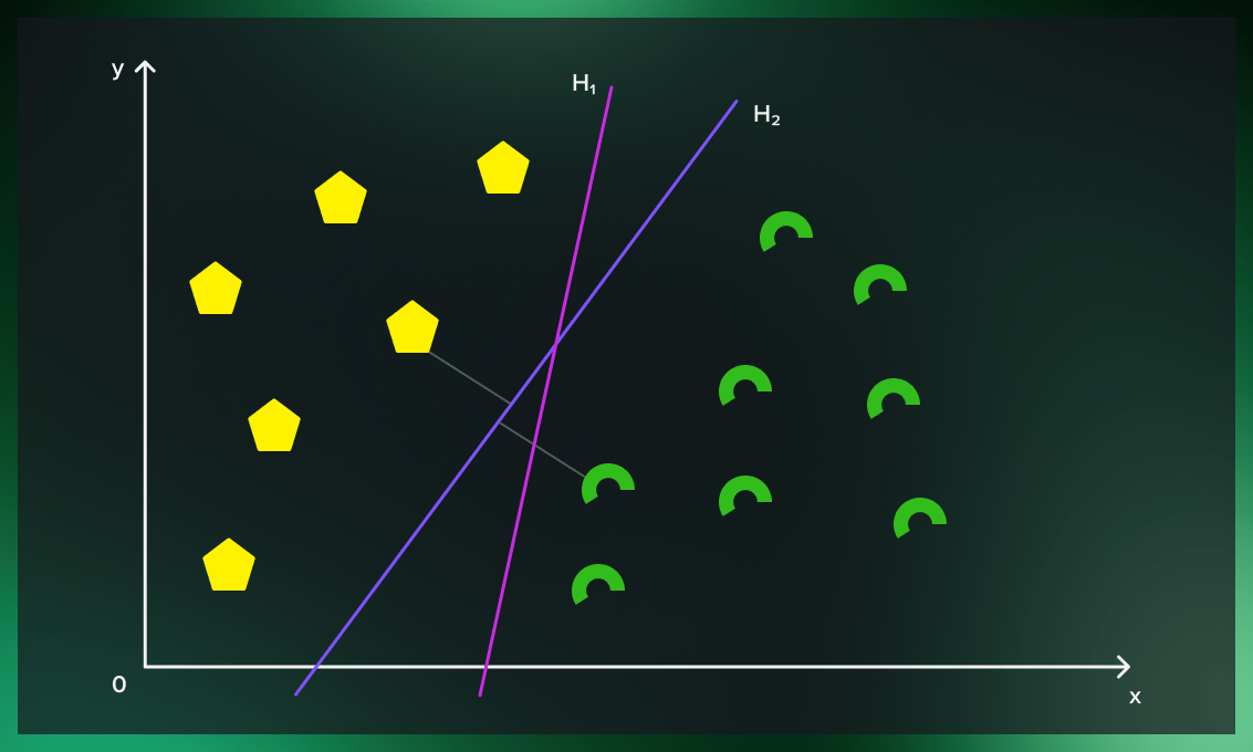
The best possible line that we can draw from the data in the training set is the one that has the greatest distance to the boundary points of each class. In our example, it’s H2.
Then, when we can use this line to classify points to each of these classes. The points that fall on the “yellow side” of the line will be classified as yellow, the points that fall on the “green side” will be classified as green. For this reason, we call it a decision boundary.
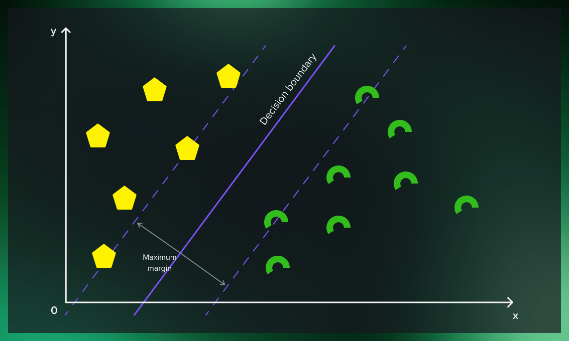
Let’s look at the two pictures above to understand how we chose the decision boundary.
First, we only pay attention to the points on the boundary between two classes and can safely forget about many others.
Now we perform a calculation. We linearly connect each pair of points on opposite sides, and the center of this line is equidistant from the classes on the boundary lines. These support points on the boundary lines are actually the sequence containers representing arrays. From now on, we will call them support vectors.
Finally, the line formed based on these middle points is our boundary line. In our example, it is a straight line, but it also can be a curve. We’ll see how that is possible later.
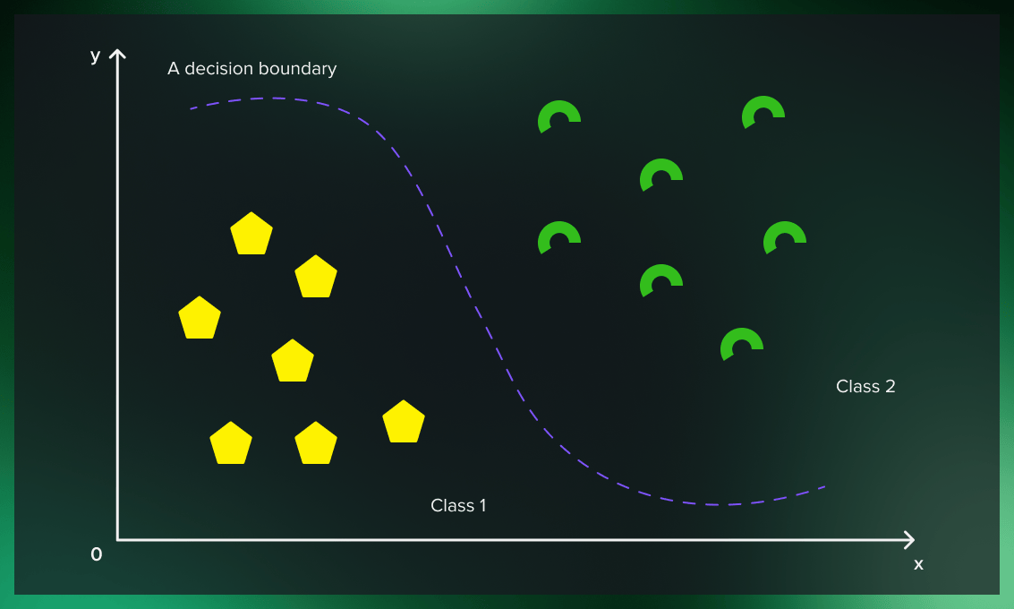
As with any supervised ML case, after training the model, we need to measure the quality of the model’s performance with a test set. After successful verification, the model can work with raw data.
If you want to go deeper into the mathematical foundation of the topic, this detailed explanation will be helpful.
Hard margin vs. soft margin in support vector machines
In the example above, we discussed a case where the points from the two classes are clearly separated. There, we worked with what’s called a hard margin.
In cases where it’s complicated to build a decision boundary without misclassifying some of the boundary points, we have to loosen the rules by introducing a soft margin.
What does a hard margin mean?
The hard margin means that the SVM is very rigid in classification and tries to perform extremely well in the training set, covering all available data points. This works well when the deviation is insignificant, but can lead to overfitting, in which case we would need to switch to a soft margin.
What does a soft margin mean?
The idea behind the soft margin is based on a simple assumption: allow the support vector classifier to make some mistakes while still keeping the margin as large as possible.
If we want a soft margin, we have to decide how to ignore some of the outliers while still getting good classification results. The solution is to introduce penalties for outfitting that are regulated by the C parameter (as it’s called in many frameworks).
Which margin to choose?
We use an SVM with hard margin when data is evidently separable. However, we may choose the soft margin when we have to disregard some of the outliers to improve the model’s overall performance.
C hyperparameter for SVM turning
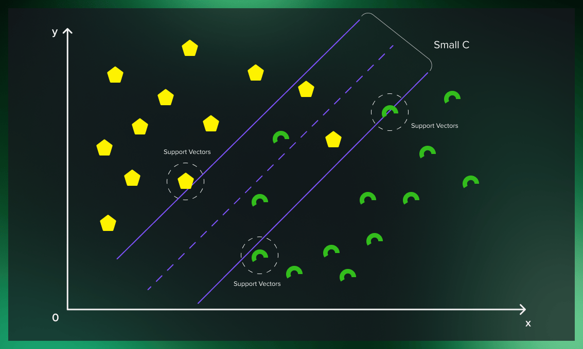
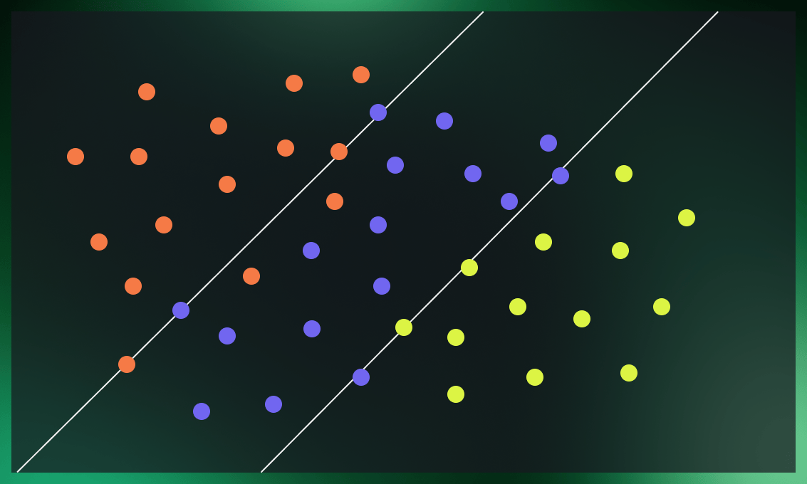
The C hyperparameter is relevant in the case of soft margin. For each misclassified data point, it applies a penalty. When C is low, choosing a decision boundary with a large margin can lead to more misclassifications because the penalty for misclassified points is low. When C is large, the support vector machine model tries to reduce the number of misclassified examples due to the high penalty, and this results in a decision boundary with a narrower margin. Not all misclassified points receive the same penalty. The further a misclassified point is from the boundary, the larger penalty it gets.
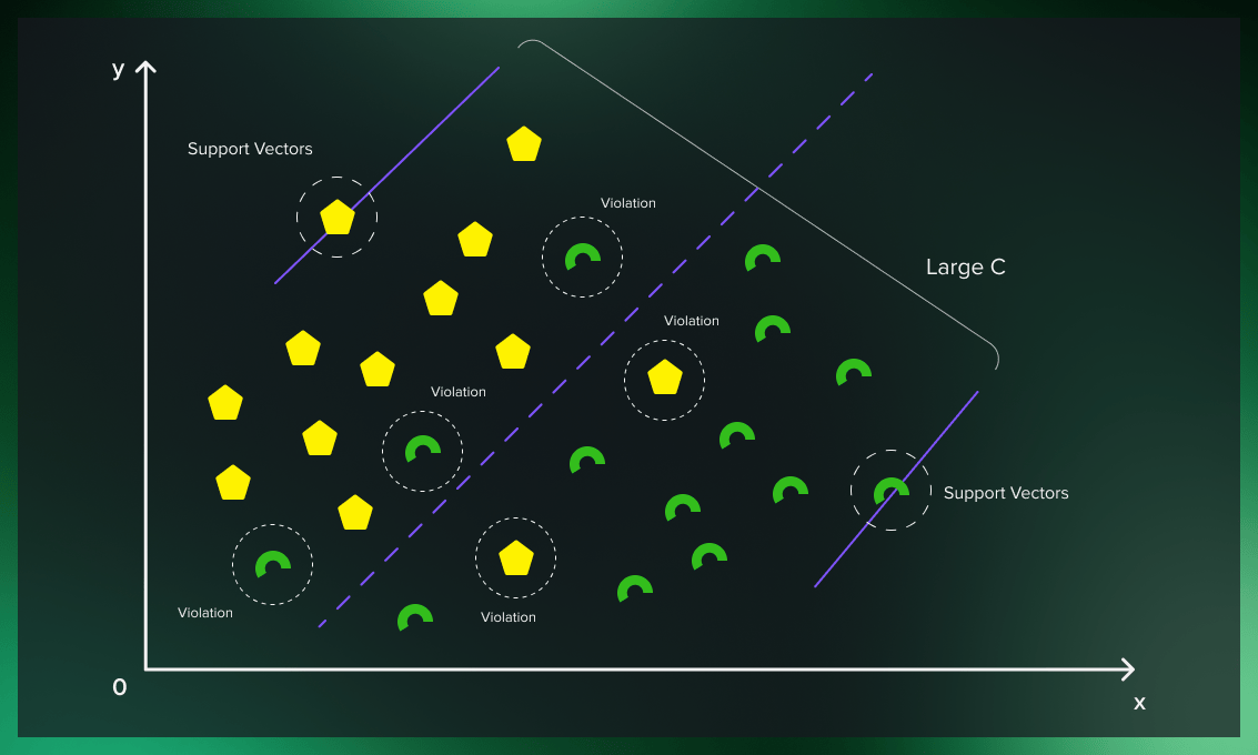
Thanks to soft margins, the model can violate the support vector machine’s boundaries to choose a better classification line. The lower the deviation of the outliers from the actual borders in the soft margin (the distance of the misclassified point from its actual plane), the more accurate the SVM road becomes. Choosing the correct soft margin value ensures that the support vector machine has the right balance between clean boundaries and generalizability.
Applying SVM to nonlinear data
Now, let’s look at more complicated cases where data cannot be separated with a line. What should we do if the dataset’s yellow tags are mixed with the green ones as in the picture below?
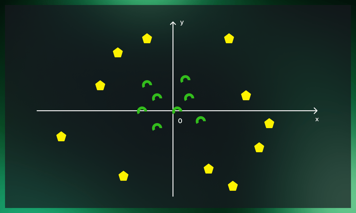
The solution is to add a third dimension to data.
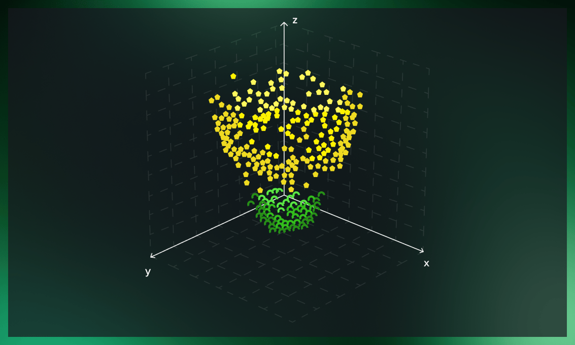
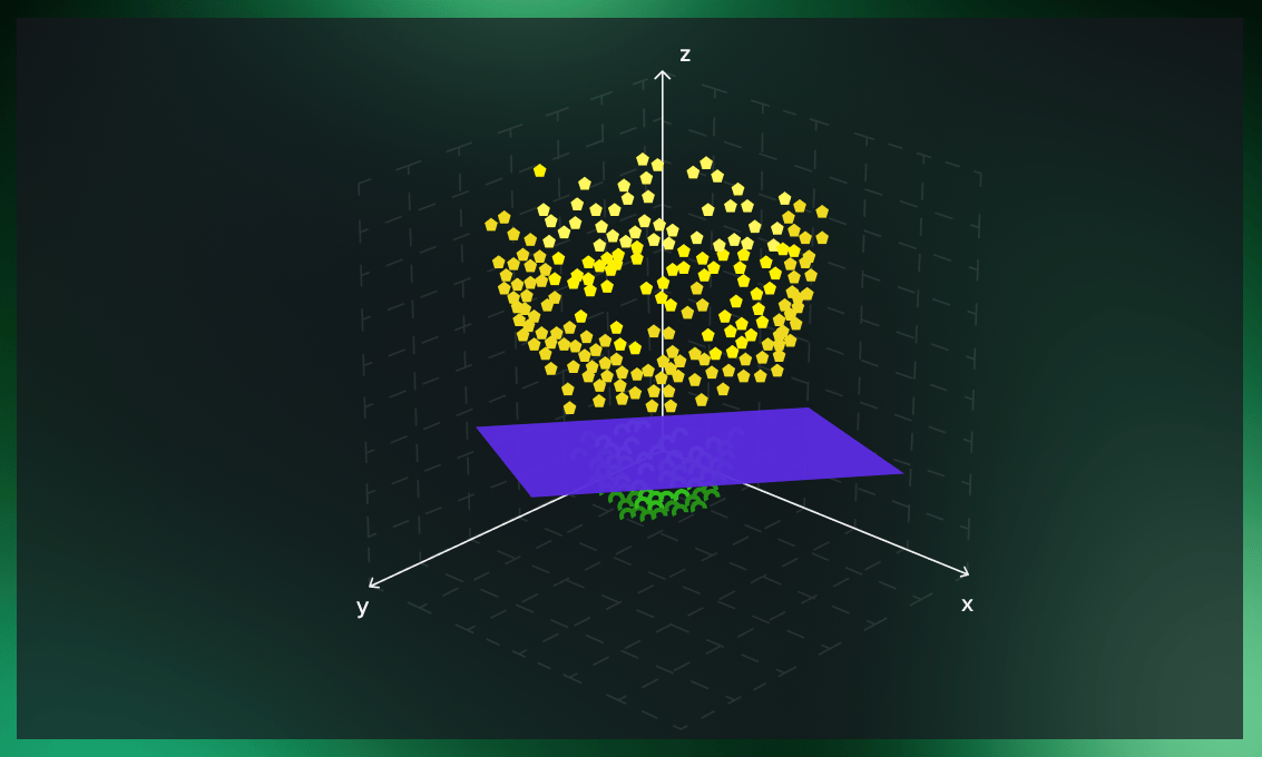
If we embed data in a higher-dimensional feature space, it’s possible to find a classifier to separate the two classes. This is done by what’s called a kernel function.
Kernel functions
To add more dimensions to the dataset, we use a kernel function.
A simple example of a kernel function is a polynomial kernel, which builds a new dimension for the dataset based on polynomials of original variables.
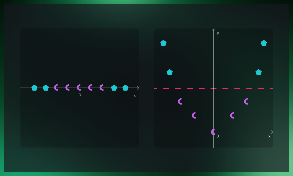
Let’s look at an example. On the picture on the left, the dataset’s classes lie in a straight line. The picture on the right shows the same dataset after we added an extra dimension to it (by setting the other axis value to be the square of the values of points), which makes the data points linearly separable.
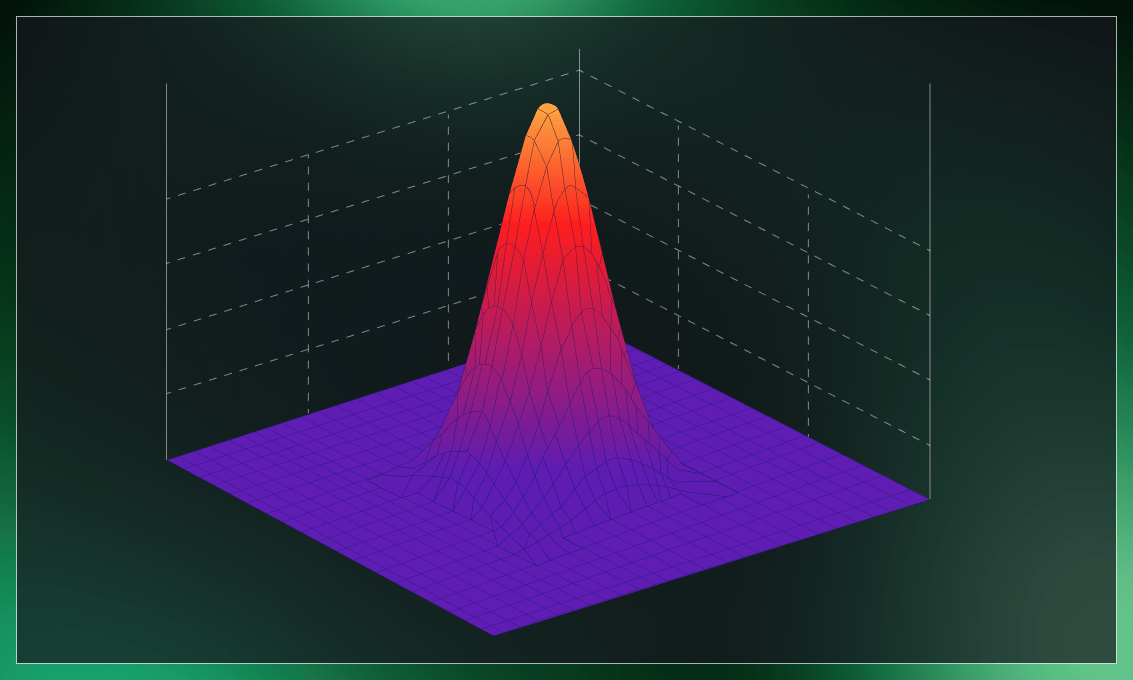
Another popular kernel is Gaussian RBF. To make classes linearly separable, it uses the radial basis function, the value of which solely depends on the distance between a fixed point and the input. For two points x1 and x2, the RBF kernel function calculates their similarity, or how close they are to each other.
To improve the performance of a kernel function, we can introduce a tuning parameter called gamma.
The gamma parameter of the RBF controls the radius of influence of a single training point. A large similarity radius, indicated by low gamma values, results in more points being grouped. At high gamma values, points must be quite close to each other to be grouped (or assigned to a class). As a result, overfitting is more common in models with very high gamma values. The concept is better explained by the following visualizations.
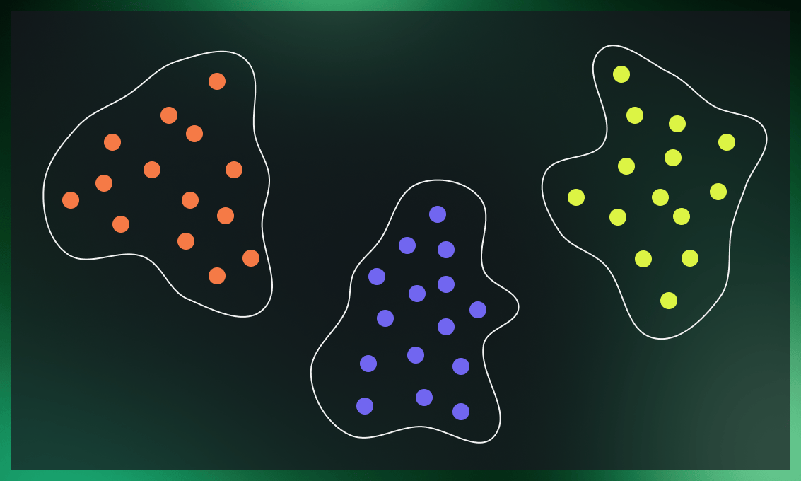
Watch this video to learn more about the application of kernels in support vector machines.
Advantages of support vector machines
Resilient to overfitting
Except for the points closest to the plane (support vectors), most of the remaining data becomes redundant. When working with the boundary points, we can intentionally allow some outliers to be misclassified to see the big picture and determine the optimal hyperplane.
Simplified calculation
Once the hyperplane is built, we can assign a class to the data points located in the classified area without the need to calculate the distances between each point.
The SVM algorithm doesn’t work well in the following situations:
- The dataset contains a lot of classes.
- The dataset contains a lot of noise.
- The target classes overlap.
Support vector machine use cases
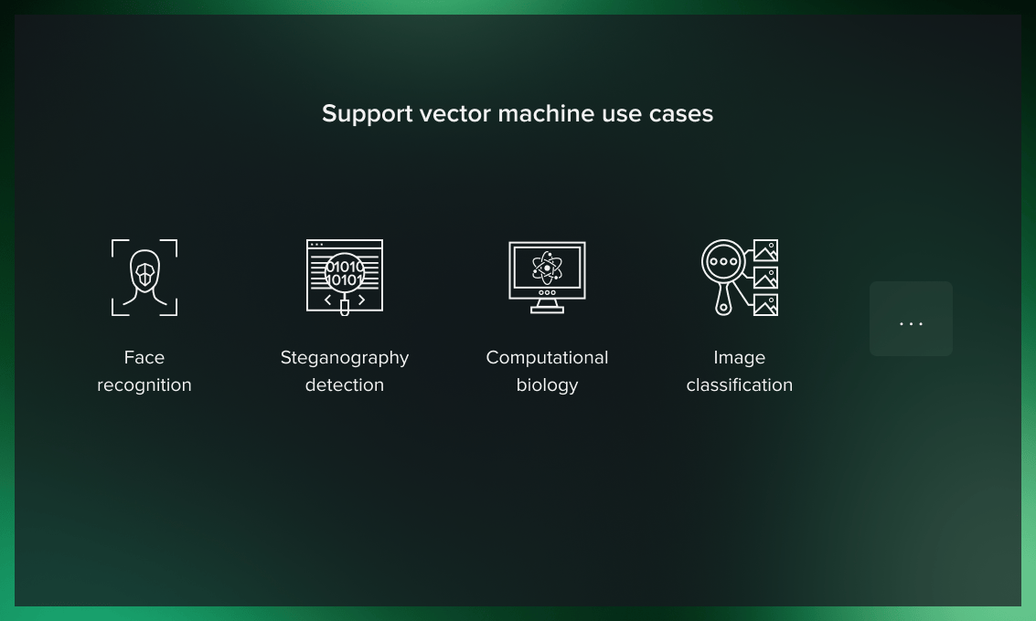
The support vector machine algorithm is widely used despite the development of more sophisticated machine learning techniques, such as deep neural networks. The reason is that the model trains quickly, has minimal processing requirements, and enables you to teach the algorithm based on a limited amount of data points rather than computing the whole training data set.
Some of the common applications of support vector machines are described below.
Computational biology
The detection of protein remote homology is a common issue in computational biology. In recent years, SVM algorithms have been extensively applied for solving this problem. These algorithms are widely used for biological sequence identification, classifying genes, predicting patients’ diseases based on their genes, etc.
Discover how Serokell’s biotech development services can enhance the efficiency of computational biology tools.
Steganography detection
With the help of SVMs, you can tell whether a digital image has been altered or contaminated. The algorithm can detect unauthorized data and watermarks illegally embedded into official documents. The support vector machine separates the individual pixels and stores the data in different datasets, making it easy to analyze.
Face recognition
The SVM classifier divides the elements of the image into face and non-face categories. First it is inputted training information for n × n pixels with face (+1) and non-face (-1) classes. Then it separates the features of each pixel into the face or non-face categories. Based on the pixel brightness, it draws a square frame around the faces and classifies each image.
Text categorization
Using training data, the support vector machine classifies documents into many categories, including news stories, emails, and web pages. For example, you can group news into “business” and “movies” or classify web pages into personal home pages and others. For that, a score is calculated for each document and compared to a given threshold. Documents are then assigned to particular categories if their score exceeds a specific value. If the value is below the threshold, the document is defined as a general one.
Image classification
SVMs can classify images more accurately compared to traditional query-based refinement systems.
Surface categorization
SVMs are used to determine textures. The algorithm performs well in categorizing surfaces in photographs as smooth or rough.
Handwriting recognition
SVMs are used to read handwritten characters for data entry and signature verification.
Geoscience
The SVM is successfully employed in the analysis and modeling of geospatial and spatiotemporal environmental data.
Watch the video below as a recap on how the support vector machine works and what applications it has.
Conclusion
SVMs are easy to implement and interpret. They provide high accuracy with less effort and computation. In addition to working on its own, the algorithm is a powerful machine learning tool to lay the basis for further investigation by neural networks. The support vector machine classifier is essential for developing applications that use predictive models and can be used in any domain.





.jpg)
.jpg)