The chronology of events, the ebb and flow of stock markets, the rhythm of the seasons—the world, as we know it, is rich with patterns and sequences that unfold over time. Time series analysis, which blends statistical and ML techniques, offers the means to analyze and interpret time-dependent datasets.
It’s essential in many sectors, from finance and economics, where it aids in predicting stock market trends, to meteorology, where it assists in weather forecasting, and even in the healthcare domain, where it is used to analyze patterns in patient vital signs.
In this blog post, we delve into the concepts of time series analysis in machine learning.
What is time series analysis?
Time series analysis is a distinct method of evaluating a chain of data elements collected over a certain time period. It entails documenting data at regular time intervals throughout a specified duration, rather than sporadic or random data recording. However, this analysis transcends simple data collection over time.
We employ time series analysis when statistical methods are ineffective and cannot be applied due to model limitations.
Time series analysis acknowledges that data points collected sequentially over time may exhibit inherent patterns or structures, such as autocorrelation, trends, or seasonal variations, which need to be considered and incorporated into the analysis.
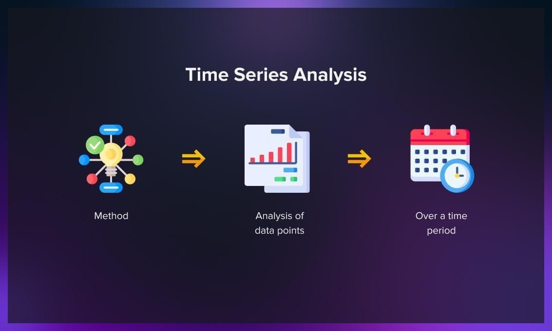
What differentiates time series data from other types is its ability to illustrate the evolution of dependencies over time. To put it simply, time stands as a significant factor as it depicts how the data modifies with each data point and affects the final outcome. It contributes an extra layer of information and establishes a sequence of dependencies among the data.
Time series analysis typically necessitates a substantial amount of data points to ensure uniformity and dependability. A vast dataset guarantees a representative sample size and enables the analysis to sift through the noise in the data. It ensures that identified trends or patterns are not anomalies and can account for any seasonal variation. Additionally, time series algorithms are an effective tool for predictive analytics, allowing future data to be anticipated based on historical data.
Why do you need time series analysis?
Time series helps organizations gain insights into the factors driving trends and recurring patterns over time. By exploring data visualizations, you can identify seasonal trends and delve into the underlying reasons behind these patterns. Advanced analytics platforms offer more than traditional line graphs, providing interactive and comprehensive visual representations.
There’s also time series forecasting, a component of predictive analytics, which allows businesses to make informed predictions about future events. By identifying patterns such as seasonality and cyclic behavior within the data, you can gain a deeper understanding of data variables and improve the accuracy of their forecasts. This enables better decision-making and planning based on anticipated changes in the data.
Watch this video to learn more about the potential of time series forecasting.
What is time series data?
Time series data consists of observations collected through repeated measurements over a period of time. These observations can be graphically represented, with time typically being one of the axes on the graph.
Time series metrics specifically refer to data points that are tracked at regular time intervals. For example, a metric could represent the daily inventory sales in a store, indicating how much inventory was sold from one day to the next.
The ubiquity of time series data is due to the fact that time is a fundamental component of nearly all observable phenomena. In our increasingly connected and sensor-laden world, systems equipped with sensors continuously generate a steady stream of time series data.
What sets time series data apart?
Time series data is immutable due to its sequential nature. It is typically recorded as new entries appended to the existing data, maintaining the order of events. Unlike relational data, which is often mutable and subject to updates in a transactional manner, time series data remains unchanged and retains its historical sequence.
For instance, in a relational database, an order for an existing customer would update multiple tables, whereas in time series data, new entries simply reflect the occurrence of events without altering previous data.
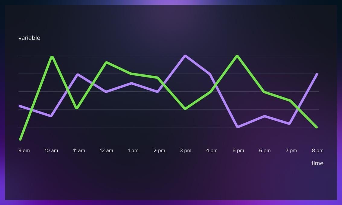
What sets time series apart from other data types is its serial dependence. This refers to the relationship between data at different points in time, indicating a degree of autocorrelation.
While all events occur within the framework of time, not all events are necessarily time-dependent. Time series data extends beyond chronological sequencing; it encompasses events where the value increases with the addition of time as an axis. Time series data can exist at various levels of granularity, spanning from microseconds to nanoseconds.
What are the qualities of time series data?
Time series data has distinct characteristics that must be considered when modeling and analyzing it. These characteristics include:
Time dependence
Time series data is inherently dependent on time. Each observation represents a data point at a specific moment in time, and subsequent observations are influenced by previous ones.
Trend
One of the key characteristics of this type of data is the presence of a trend. Trends are gradual, long-term changes in the data’s values over time. It could be an upward trend (indicating growth or increase) or a downward trend (indicating decline or decrease). Identifying and accounting for the trend is essential in time series forecasting models.
Seasonality
It often exhibits seasonal patterns or effects. These patterns occur regularly within specific time intervals, such as seasons, quarters, or months. Seasonality can be influenced by factors like holidays, weather changes, or business cycles. Properly capturing and incorporating seasonality into forecasting models is crucial for accurate predictions.
Noise
Another characteristic of time series data is the presence of random error or noise. Noise represents unpredictable fluctuations or variability in the data that can obscure underlying patterns. Accounting for and minimizing the impact of noise is necessary to ensure the accuracy of forecasting models.
What are time series data types?
Time series data can be classified into two categories: stationary and non-stationary data.
Stationary data
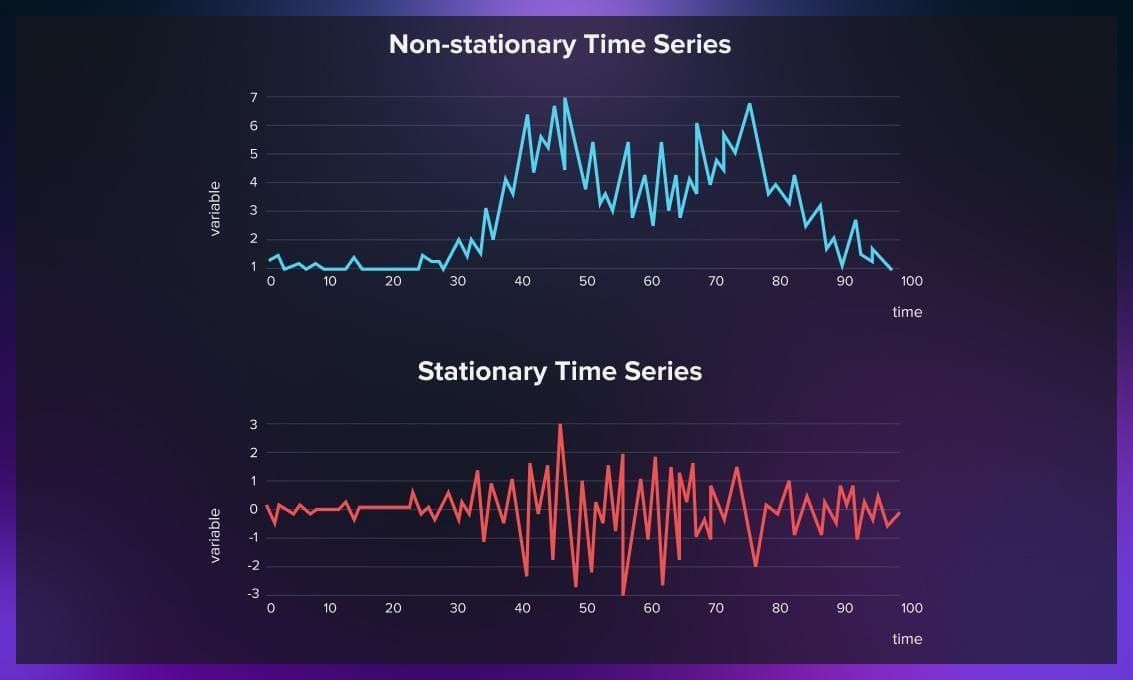
Stationary time series data refers to data in which the statistical properties remain constant over time. It lacks any discernible trend, seasonality, or patterns that would cause significant changes in these statistical properties. The variability in the dataset is primarily attributed to random error.
For instance, the number of visitors to a library on random weekdays can be considered stationary data, as it does not exhibit noticeable trends or seasonality. Similarly, the daily closing price of a stable blue-chip stock, devoid of significant trends or seasonality, can also be categorized as stationary data.
Non-stationary data
On the other hand, non-stationary time series data displays either a trend or a seasonal effect. Random error alone does not account for the variability in such data sets. To accurately model and forecast non-stationary time series data, additional preprocessing steps like detrending or differencing are necessary to eliminate the non-stationarity. Here are a few examples of non-stationary time series datasets:
- Annual sales figures of a company experiencing steady growth over the years, indicating a clear trend.
- Monthly temperature readings of a city exhibiting a seasonal pattern as temperatures rise and fall with the changing seasons.
- Stock prices of a new startup that has witnessed significant growth within a short period, showing a pronounced upward trend over time.
Non-stationary time series data necessitates appropriate treatment to remove the non-stationarity before accurate modeling and forecasting can be achieved. By distinguishing between stationary and non-stationary time series data and employing the appropriate techniques, you can gain meaningful insights and make reliable predictions.
What are the steps of time series analysis?
To conduct this analysis, you need to follow these steps:
1. Data collection and cleansing
Gather the required data and ensure it is free from errors or missing values.
2. Time-based visualization
Create visualizations that depict the relationship between time and the key features of interest.
3. Assessing stationarity
Determine the stationarity of the time series by examining its statistical properties over time.
4. Exploratory analysis Generate charts and graphs to gain insights into the nature and patterns of the time series.
5. Model development
Build various models such as Autoregressive (AR), Moving Average (MA), Autoregressive Moving Average (ARMA), and Autoregressive Integrated Moving Average (ARIMA) to capture the dynamics of the time series.
6. Extracting insights from predictions
Analyze the predictions made by the models to gain meaningful insights and draw conclusions about the underlying patterns and trends in the time series.
Pre-processing data for analysis
In order to accurately predict the values of a time series, it is crucial to eliminate values that fall outside of a predetermined range and create abnormal fluctuations in the series. For instance, a year-long price series for petrol ranges from $0,99 to $1,05. However, due to a supply shortage, the price temporarily exceeded $1,2 for a few days. Such fluctuations can introduce uncertainty in prediction models, and it is unnecessary to include them in the modeling process. To address this, we can employ filters to remove such anomalous values.
Here are some commonly used filters:
- Moving average filter: It smooths the time series by calculating the average of neighboring data points within a specified window. It helps to highlight the underlying trends or patterns in the data.
- Exponential smoothing filter: Exponential smoothing is a popular filter that assigns exponentially decreasing weights to past observations. It places more emphasis on recent data points while gradually decreasing the influence of older points. This filter is particularly useful for capturing short-term trends.
- Savitzky-golay filter: It is a type of polynomial smoothing filter that can effectively remove noise. It fits a polynomial to a sliding window of data points and estimates the filtered value based on the polynomial coefficients. This filter is often used for preserving important features of the signal while reducing noise.
- Median filter: The median filter replaces each data point with the median value within a specified window. It is robust to outliers and can effectively remove impulse noise or sharp spikes in the time series.
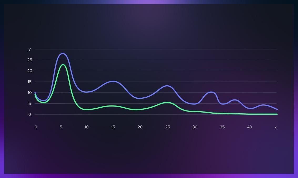
The choice of filter depends on the characteristics and the specific requirements of the analysis. It is often beneficial to experiment with different filters and window sizes to find the most suitable approach for your particular dataset.
What are the types of time series analysis in machine learning?
Time series analysis encompasses various categories or approaches to analyzing data, which can sometimes require the development of complex ML models. However, it is important to recognize that it is impossible to account for all variations in the data, and a specific model cannot be generalized to every sample. Overly complex models or models attempting to address multiple aspects can lead to a lack of fit. Overfitting occurs when models fail to distinguish between random error and genuine relationships, resulting in skewed analysis and inaccurate forecasts.
The machine learning models used in time series analysis include:
- Classification
This approach aims to identify and assign categories or labels to the data based on specific criteria or characteristics.
- Curve fitting
This technique involves plotting the data points along a curve to analyze and understand the relationships between variables within the data.
- Descriptive analysis
Descriptive analysis focuses on identifying patterns, trends, cycles, or seasonal variations within the time series database.
- Explanatory analysis
Explanatory analysis seeks to understand the data and the relationships among variables, exploring cause-and-effect dynamics.
- Exploratory analysis
Exploratory analysis aims to uncover and highlight the main characteristics of the time series dataset, often using visual representations.
- Forecasting
Forecasting involves predicting future data points based on historical trends. It utilizes historical data as a model for future data, enabling the estimation of potential scenarios.
- Intervention analysis
Intervention analysis examines how specific events or interventions can impact the data, studying the effects of these interventions on the time series.
- Segmentation
Segmentation involves dividing the data into segments or subsets to reveal underlying properties or patterns within the original data source.
Advanced techniques in time series analysis
Time series analysis offers advanced techniques that enhance the understanding and prediction of temporal data. These techniques enable analysts to extract more nuanced insights and improve forecasting accuracy. Below we explore some advanced analysis techniques.
Transformers
Transformers, originally designed for natural language processing, have been extended to various domains, including time series analysis. The standard approach is to adapt Transformer-based architectures such as BERT, GPT, or Transformer Encoder for this purpose.
The process involves the following steps:
- preprocessing data into tokenized input-output pairs;
- encoding it and choosing a suitable Transformer-based architecture, for example, the Transformer Encoder;
- training the model with appropriate loss functions and validating hyperparameters;
- evaluating the model’s performance on the test set;
- handling variable-length sequences using padding or masking techniques.
Seasonal decomposition
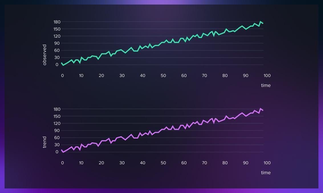
Seasonal decomposition involves breaking down a time series into its underlying components: trend, seasonality, and residual (or error) component. This technique helps identify and isolate the seasonal patterns within the data, providing a clearer understanding of the underlying dynamics.
Exponential smoothing models (Holt-Winters, ARIMA-ETS)
Exponential smoothing models, such as Holt-Winters and ARIMA-ETS (Error, Trend, Seasonality), are powerful tools for time series forecasting. These models take into account the trend and seasonality present in the data and provide reliable predictions. Holt-Winters models are particularly effective in capturing seasonal variations, while ARIMA-ETS models handle more complex patterns.
Long Short-Term Memory (LSTM) networks
LSTM networks, a kind of recurrent neural network (RNN), have gained popularity in time series forecasting. LSTM models can capture long-term dependencies in sequential data and effectively handle non-linear relationships. These networks excel in capturing complex patterns and are widely used in various domains, including finance, energy, and natural language processing.
Model evaluation and performance metrics
Assessing the performance of time series models is crucial for understanding their accuracy and reliability. Various performance metrics, such as mean squared error (MSE), mean absolute error (MAE), and root mean squared error (RMSE) help evaluate the models’ effectiveness. Additionally, graphical techniques like residual analysis, forecast error plots, and quantile-quantile plots provide insights into model performance and any residual patterns.
Watch this video to learn more about forecasting in machine learning:
Limitations of time series analysis
When doing a time series analysis, we must consider its four pivotal components—trend, seasonality, cyclicity, and irregularities—to accurately interpret results and form future predictions. While the former two are deterministic, the latter two components pose more of a challenge. For this reason, we need to isolate random events to identify and predict potential patterns.
Also, we have to be careful when extrapolating from a limited sample size. For example, determining the typical running times for a customer requires the examination of running habits across a broad base of customers. Forecasting future data points can prove difficult if the preliminary stages of data processing were not carried out properly. There’s also a risk of unexpected anomalies .
The reliability of predictions generally diminishes the further into the future they extend. This is evident when we consider the often inaccurate nature of a 10-day weather forecast. Likewise, time series analysis cannot offer definitive future predictions, but rather probabilities for specific outcomes. For instance, while we cannot definitively assert that a health app user will achieve over 10,000 steps on a given Sunday, we can state that there is a high probability, or a 95% certainty, according to historical data.
ML tools, libraries and packages for time series analysis
Now, let us explore a selection of tools, packages, and libraries that can assist in your project. As many projects related to time series analysis in data science and machine learning are often carried out using Python, we’ll mainly focus on tools supported by this programming language.
sktime
Sktime is a Python framework that focuses on time series data analysis. Its comprehensive tools enable efficient processing, visualization, and analysis of time-series data. With a user-friendly design and extensibility in mind, sktime facilitates the seamless implementation of new time-series algorithms.
Sktime extends the scikit-learn API, encompassing all essential methods and tools for solving time series regression, prediction, and classification problems. Apart from offering specialized machine learning algorithms, the library also incorporates conversion methods specifically designed for time-series data. These unique features distinguish Sktime from other existing libraries.
Datetime
Datetime is a Python module that facilitates working with dates and times by providing a range of methods and functions. This module enables you to handle various scenarios, including representing and comparing dates and times and performing calculations.
When it comes to working with a time series database, this tool simplifies the process by allowing users to transform dates and times into objects and manipulate them easily. For instance, with just a few lines of code, we can convert between different DateTime formats, add or subtract a specified number of days, months, or years to date, or calculate the time difference in seconds between two time objects.
Tsfresh
Tsfresh is a Python package that automates the computation of a wide range of features. This package enables the systematic extraction of meaningful features from time series data.
Tsfresh incorporates a filtering procedure to ensure the extracted features’ relevance. This procedure evaluates each characteristic’s explanatory power and significance in the context of regression or classification tasks.
The package offers several advanced time series features, including:
- Fourier transform components
- Wavelet transform
- Partial autocorrelation
Statsmodels
Statsmodels is a comprehensive Python package that offers a collection of classes and functions to estimate various statistical models, conduct statistical tests, and perform statistical data analysis.
Statsmodels provides a convenient method for time series decomposition and visualization. With this package, we can effortlessly decompose any time series and examine its components, including trend, seasonal patterns, and residual or noise.
pmdarima
Pmdarima is a Python library designed for the statistical analysis of time series data built upon the ARIMA (AutoRegressive Integrated Moving Average) model. It offers tools for analyzing, forecasting and visualizing time series data. Additionally, pmdarima provides specialized functionality for working with seasonal data, such as a seasonality test and a tool for seasonal decomposition.
ARIMA is a popular forecasting model that enables us to predict future values based solely on the time series’ historical values without requiring additional information.
Pmdarima is a convenient wrapper over the ARIMA model, incorporating an “auto” function that automatically determines the best hyperparameters (p, d, q) for the ARIMA model. Notable features of the library include:
- Similar functionality to R’s “auto.arima” capability.
- A collection of statistical tests to assess stationarity and seasonality in time series.
- Various transformers and featurizers, both endogenous and exogenous, including Box-Cox and Fourier transformations.
- Utilities for operations, such as differencing and inverse differencing.
- A diverse collection of built-in datasets for prototyping and providing examples.
- Seasonal decomposition tools.
- Utilities for cross-validation.
PyCaret
PyCaret is a Python library for machine learning that offers a low-code approach, making it easier to automate machine learning workflows. With PyCaret, you can significantly accelerate the experiment cycle and enhance productivity.
Compared to other open-source machine learning libraries, PyCaret stands out as a low-code alternative that can replace lengthy code blocks with just a few lines. This streamlined approach ensures faster and more efficient experimentation. PyCaret is a Python wrapper for various machine learning libraries and frameworks, including scikit-learn, XGBoost, LightGBM, CatBoost, spaCy, Optuna, Hyperopt, Ray, etc.
While PyCaret is not primarily focused on time series forecasting, it does offer a dedicated module for this purpose. Although the module is currently in pre-release mode, you can try it out by installing PyCaret with the “–pre” tag.
The PyCaret time series module aligns with the existing API and comes fully equipped with various functionalities. These include statistical testing, model training and selection (with 30+ algorithms), model analysis, automated hyperparameter tuning, experiment logging, and even deployment on cloud platforms.
Time series analysis applications
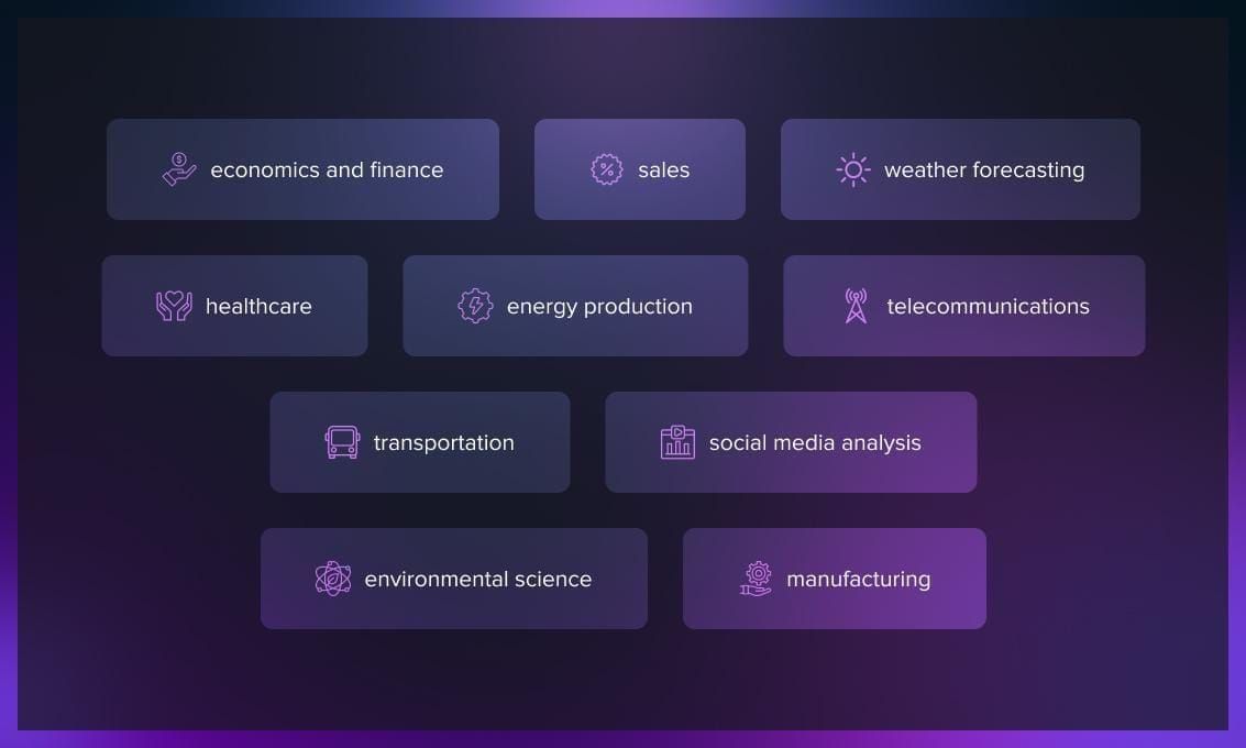
The application of time series analysis is vast and versatile. In essence, any scenario where data are collected over time and future forecasting is required can potentially benefit from time series analysis. In this section, we explore some of the most common:
Economics and finance
Forecasting stock prices, market trends, and economic factors are vital tasks in this field. Economists and financial analysts use time series analysis to model and forecast GDP, unemployment rates, interest rates, and stock prices.
Sales
Businesses use time series forecasting to predict future sales, demand, and revenue. This data is crucial for budgeting, planning, and inventory management.
Weather forecasting
Meteorologists predict future weather conditions, including temperatures, rainfall, and wind speed. This information is vital for planning activities in agriculture, tourism, construction, and many other sectors.
Healthcare
Time series modeling is used in healthcare to predict disease outbreaks, patient outcomes, and healthcare resource needs, among other things. For example, during the COVID-19 pandemic, this analysis was used to predict the spread of the virus and the need for hospital resources.
Energy production
The production and consumption of energy can be modeled and forecasted using time series analysis. This includes predictions about the need for electricity in response to weather patterns or the productivity of wind or solar power plants.
Telecommunications
It can be used to predict data traffic, network incidents, and resource utilization. It’s used to optimize network performance and plan infrastructure development.
Transportation
In the transportation industry, time series analysis is used for traffic prediction, optimizing routes, and planning infrastructure development.
Social media analysis
Social media posts can be analyzed as a time series to identify trends, detect the spread of information, sentiment analysis, and predict future post volumes.
Environmental science
Ecologists and environmental scientists can track changes in ecosystems over time, predicting things like animal population sizes, levels of pollution, or the impact of climate change.
Manufacturing
In manufacturing, time series analysis can be used to predict equipment failures and maintenance needs, which can help to prevent downtime and improve efficiency.
Conclusion
Time-series analysis, with its nuanced exploration of temporal data, is a powerful tool for predicting future trends, seasonality, and cyclicity. Yet, it has limitations, and imperfections in data processing and unpredictable irregularities can impact the accuracy of forecasts. Hence, predictions are not absolutes but probability distributions. While time series analysis can’t eliminate uncertainties, it illuminates hidden patterns. It offers probabilistic foresight, thus providing a robust foundation for informed decision-making in various fields, from finance to healthcare and beyond.


.jpg)
.jpg)


.jpg)
