Backpropagation is a fundamental component of deep learning for neural networks. Its development has significantly contributed to the widespread adoption of deep learning algorithms since the early 2000s. In this post, we explore the essential concepts associated with this method, as well as its applications and history.
What is forward and backward propagation?
Forward propagation in neural networks refers to the process of passing input data through the network’s layers to compute and produce an output. Each layer processes the data and passes it to the next layer until the final output is obtained. During this process, the network learns to recognize patterns and relationships in the data, adjusting its weights through backpropagation to minimize the difference between predicted and actual outputs.
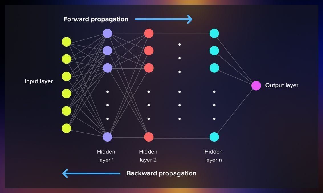
The backpropagation procedure entails calculating the error between the predicted output and the actual target output while passing on information in reverse through the feedforward network, starting from the last layer and moving towards the first. To compute the gradient at a specific layer, the gradients of all subsequent layers are combined using the chain rule of calculus.
Backpropagation, also known as backward propagation of errors, is a widely employed technique for computing derivatives within deep feedforward neural networks. It plays a crucial role in various supervised learning algorithms used for training this type of neural networks.
Training of a neural network involves using gradient descent, an iterative optimization algorithm for discovering a local minimum of a differentiable function. During the training process, a loss function is computed to measure the disparity between the network’s predictions and the actual values. Backpropagation enables the calculation of the gradient of the loss function concerning every weight in the network. This capability enables individual weight updates, gradually reducing the loss function over multiple training iterations.
What does the backpropagation process look like?
Backpropagation serves the purpose of minimizing the cost function by fine-tuning the neural network’s weights and biases. The extent of these adjustments hinges on the gradients of the cost function concerning these specific parameters. By computing the gradients through the chain rule, backpropagation efficiently propagates error information backward through the network. Consequently, the network can iteratively update its parameters in the direction opposite to the gradient. This iterative process enables the neural network to converge towards improved performance and accurate predictions.
The fundamental steps involved in computing the gradients of the weights in a neural network in backpropagation, are the forward and backward passes.
Forward pass
During the forward pass, the input data is propagated through the network layer by layer, starting from the input layer and moving towards the output layer. Each neuron in the network receives inputs, calculates a weighted sum of the inputs, applies an activation function, and passes the output to the next layer. This process continues until the final output is obtained. The forward pass calculates the output of the network based on the current weights.
Before we proceed to the backward pass, we need to introduce the quickest possible way to calculate the optimal weights, which is not a trivial task for complicated multiparametric networks. This is where the computational graph comes into play.
What is a computational graph?
A computational graph is a directed graph used to represent the computations performed inside a model. The graph typically starts with inputs like data (X) and labels (Y). As we move from left to right in the graph, we encounter nodes representing fundamental computations involved in computing the function. For instance, there are nodes for matrix multiplication between input (X) and weight matrix (W), a red node for hinge loss (used in SVM classifiers), and a green node for the regularization term in the model. The graph concludes with an output node representing the scalar loss (L) to be computed during model training. While this computational graph might seem simple for linear models due to the limited number of operations, it becomes more complex and crucial for intricate models with multiple computations.
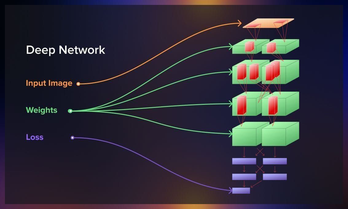
And when we go backwards, with the goal of calculating the optimal loss function, a computational graph is the means to an optimal solution, which significantly reduces the required computations.
The process is explained in detail in this whitepaper.
At each node, reverse-mode differentiation merges all paths that originated at that node. We do not need to evaluate all possible combinations of the weights’ mutual influence, but thanks to derivatives, we can have the proper coefficients by computing the backward operation for each of the nodes only once.
Backward pass
In the backward pass, the gradients of the weights are computed by propagating the error backwards through the network. It starts from the output layer and moves towards the input layer. The error is quantified by comparing the predicted output of the network with the true output or target value. The gradient of the loss function with respect to each weight is calculated using the chain rule of calculus, which involves computing the partial derivatives of the weights at each layer. The gradients are then used to update the weights of the network, aiming to minimize the loss function.
The backward pass essentially determines how much each weight contributed to the overall error and adjusts them accordingly. By iteratively performing forward and backward passes, the network learns to adjust its weights, improving its ability to make accurate predictions.
Watch this video for a detailed explanation of forward and backward propagation.
What are the types of the backpropagation algorithm?
The two main types of backpropagation networks are static backpropagation, which provides instant mapping, and recurrent backpropagation, which involves fixed-point learning.
1.Static backpropagation: It is commonly used in feedforward neural networks and some convolutional neural networks (CNNs) where there is no temporal dependence between data points. The algorithm accumulates the gradients of the loss function over a batch of data points and then performs a single update to the model’s parameters. The batching process helps to take advantage of parallel processing capabilities in modern hardware, making the training process more efficient for large datasets.
This algorithm is capable of solving static classification problems, such as optical character recognition (OCR).
2.Recurrent backpropagation: Recurrent backpropagation is an extension of the backpropagation algorithm used in recurrent neural networks (RNNs). In RNNs, the data flows in cycles through a series of interconnected nodes, allowing the network to retain information from previous time steps.
Recurrent backpropagation involves propagating the error signal backward through time in the RNN. It calculates the gradients of the loss function with respect to the model’s parameters over multiple time steps, taking into account the dependencies and interactions between the current time step and the previous ones. This process enables the network to learn and update its parameters to improve its performance on tasks that require sequential or temporal dependencies, such as natural language processing, speech recognition, and time series prediction.
Why use backpropagation?
After the completion of the forward pass, the network’s error is evaluated and ideally should be minimized.
If the current error is high, it indicates that the network has not effectively learned from the data. In other words, the current set of weights is not sufficiently accurate to minimize the error and generate precise predictions. Consequently, it becomes necessary to update the neural network weights to reduce the error.
Backpropagation algorithm plays a crucial role in weight updates with the objective of minimizing the error.
Advantages of the backpropagation algorithm
Backpropagation offers several key benefits:
1. Memory efficiency
It efficiently calculates derivatives, utilizing less memory compared to alternative optimization algorithms like the genetic algorithm. This is particularly beneficial when working with large neuron networks.
2. Speed
It is fast, particularly for small and medium-sized NNs. However, as the number of layers and neurons increases, the computation of more derivatives can result in slower performance.
3. Versatility
This algorithm is applicable to various network architectures, including convolutional neural networks, generative adversarial networks, fully-connected networks, and more. Backpropagation’s generic nature allows it to work effectively in diverse scenarios.
4. Parameter simplicity
Backpropagation does not require tuning specific parameters, thereby reducing overhead. The only parameters involved in the process are associated with the gradient descent algorithm, such as the learning rate.
While working with neural networks, we can utilize different algorithms to reduce the output of the loss function and learning rate to provide more precise results. There are many alternative methods for modifying the attributes of your neural network, such as Adam (Adaptive Moment Estimation), which has been state-of-the-art for years, Nesterov Accelerated Gradient, AdaGrad, and AdaDelta.
If you wish to learn more on this point, check out this detailed description of different optimizers.
One of the most advanced algorithms for loss function optimization is the Sophia optimizer, released in May 2023 by Stanford researchers. The classical example of such optimizers is the cost function, which we explain below.
Computing backpropagation: Cost function
Cost function represents the square of the difference between the model’s output and the desired output.
When applying a neural network to millions of images with associated pixel values, we can assume predicted output and the corresponding actual values.
A smaller cost function indicates better model performance on the training data. Moreover, a model with a minimized cost function is expected to perform well on unseen data as well.
The cost function takes all the input, which can involve millions of parameters, and produces a single value. This value serves as a guide, indicating how much improvement is required in the model. It informs the model that it is performing poorly and adjustments are needed in its weights and biases. However, simply informing the model about its performance is not sufficient. We also need to provide a method to the model that allows it to minimize the error.
This is where gradient descent and backpropagation come into play, providing the means for the model to update its parameters and reduce the cost function.
Gradient descent
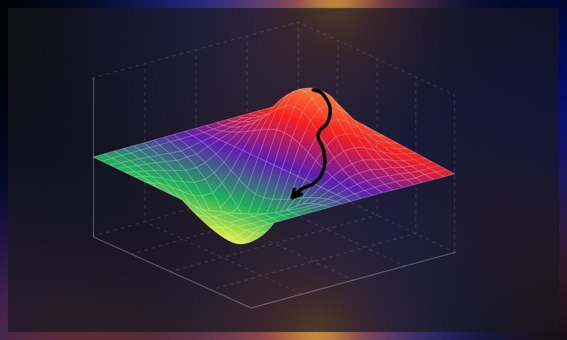
To achieve better parameter tuning and minimize discrepancies between actual and training output, we employ an intuitive algorithm called gradient descent. Currently, gradient descent is the most popular optimization strategy in machine learning and deep learning. This algorithm identifies errors and effectively reduces them. Mathematically, it optimizes the convex function by finding the minimum point.
The concept of gradient can be understood as the measurement of how a function’s output changes when its inputs are slightly modified. It can also be visualized as the slope of a function, where a higher gradient indicates a steeper slope and facilitates faster learning for the model. Metaphorically, you can liken it to descending to the bottom of a valley rather than ascending a hill. This is because it is an optimization algorithm that minimizes a given function.
Types of gradient descent
Now let’s explore different types of gradient descent.
Batch gradient descent
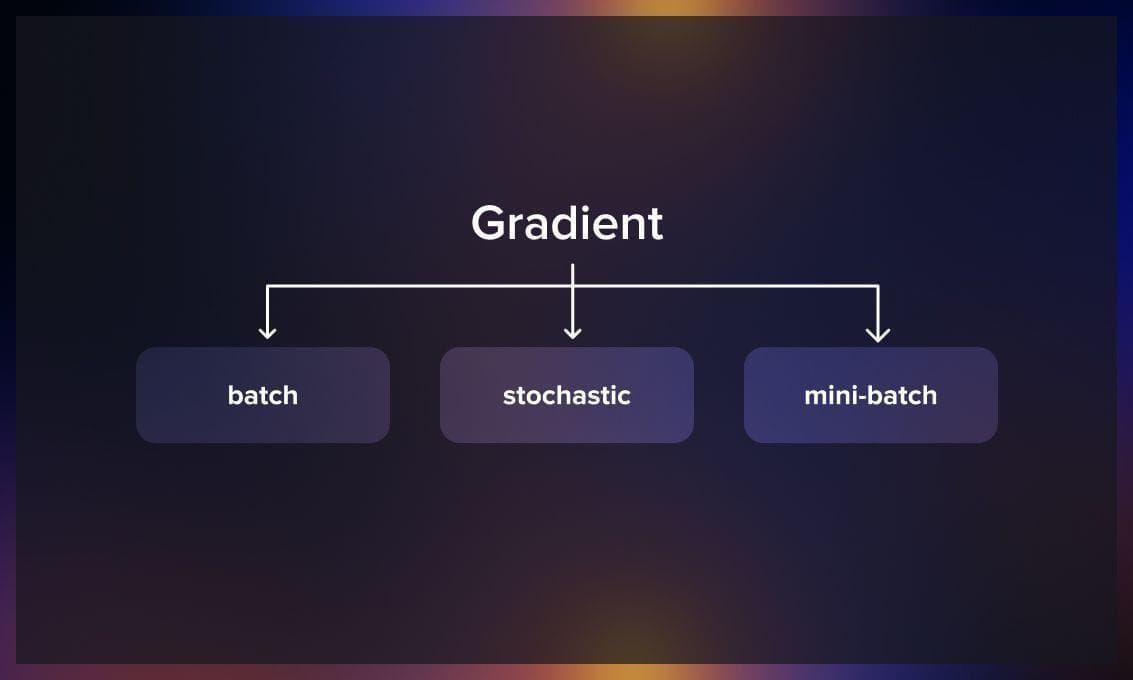
The batch size refers to the total number of training examples included in a single batch. Since it is not feasible to pass the entire dataset into the neural network at once, the dataset is divided into multiple batches or subsets.
In batch gradient descent, the complete dataset is utilized to compute the gradient of the cost function. However, this approach can be slow since it requires calculating the gradient over the entire dataset for each update. It can be challenging, especially with large datasets. The cost function is computed after initializing the parameters, and the process involves reading all the records into memory from the disk. After each iteration, one step is taken, and the process is repeated.
Mini-batch gradient descent
Mini-batch gradient descent is a commonly used algorithm that provides faster and more accurate results. The dataset is divided into small groups or batches of ‘n’ training examples. Unlike batch gradient descent, mini-batch gradient descent does not use the entire dataset. In each iteration, a subset of ‘n’ training examples is employed to compute the gradient of the cost function. This approach reduces the variance of parameter updates, leading to more stable convergence. Additionally, it can leverage optimized matrix operations, enhancing gradient computations’ efficiency.
Stochastic gradient descent
Stochastic gradient descent (SGD) updates the model’s parameters based on the gradient computed for a random subset of the data at each iteration, thus allowing for faster computation. At each iteration (or epoch) of training, a random batch of data points is selected from the training dataset. The gradient of the loss function with respect to the model’s parameters is then calculated using the selected batch. Next, the model’s parameters are updated based on the computed gradient. The update is performed in the opposite direction of the gradient to move towards the minimum of the loss function. These steps are repeated for a fixed number of iterations or until convergence criteria are met.
Backward propagation in Tensorflow and Pytorch
The backpropagation algorithm is a crucial technique used for training deep learning models.
In TensorFlow, you can use backpropagation by defining your neural network model, compiling it with an optimizer and loss function, preparing your data, and then training the model using the fit function. TensorFlow’s automatic differentiation handles the computation of gradients during training, making it easier to apply backpropagation to train complex models effectively.
To employ backpropagation in PyTorch, you need to define the neural network architecture and loss function. During the training process, data is passed forward through the network to make predictions, and then gradients are automatically computed in reverse order through the network’s layers using the backward function. These gradients are then used to update the model’s parameters using an optimization algorithm like stochastic gradient descent.
To learn more about the use of backpropagation in PyTorch, watch this tutorial:
Applications of backpropagation
Backpropagation is extensively used in training various types of neural networks and has played a significant role in the recent surge of deep learning’s popularity. But the application of backward propagation is much wider, ranging from weather forecasting to analyzing numerical stability. Here are a few examples of its application in machine learning.
Face recognition
Convolutional neural networks are the go-to technique in deep learning for image processing and recognition, often trained using the backpropagation algorithm. In a study by Parkhi, Vedaldi, and Zisserman in 2015, they developed a face recognition system using an 18-layer CNN and a database of celebrity faces. The network was trained using backpropagation across all 18 layers, with images processed in batches. The researchers used a loss function called a triplet loss to refine the network’s ability to distinguish subtle facial nuances. This involved feeding triplets of images (e.g., two images of Angelina Jolie and one of Nicole Kidman) through the network, penalizing the network for misclassifying same-person images as different and for classifying different-person images as similar. This training process continued iteratively, updating the weights of the previous layer.
NLP: Speech recognition
Backpropagation has been applied to train neural networks for various NLP tasks, including sentiment analysis, language translation, text generation, and speech recognition. Recurrent neural networks (RNNs) trained with backpropagation are commonly used for sequential data processing in NLP.
For example, Sony developed a system capable of recognizing limited commands in English and Japanese. The system uses incoming sound signals divided into time windows, applying a Fast Fourier Transform to extract frequency-based features, which are then input into a neural network with five layers. Backpropagation is employed to train these layers to understand Japanese commands, using a softmax cross-entropy loss function. The researchers were able to adapt the same network to recognize English commands through retraining, showcasing transfer learning capabilities.
Accidents prevention
The number of underground mines is increasing due to the depletion of resources on the surface. This paper offers a method to improve the prediction of post-blast re-entry time in underground mines, which is crucial for ensuring worker safety and productivity. Currently, methods like fixed-time intervals and empirical formulas are used, but they have limitations and may not be universally applicable. Backpropagation neural networks can be a solution, the authors suggest.
History of backpropagation
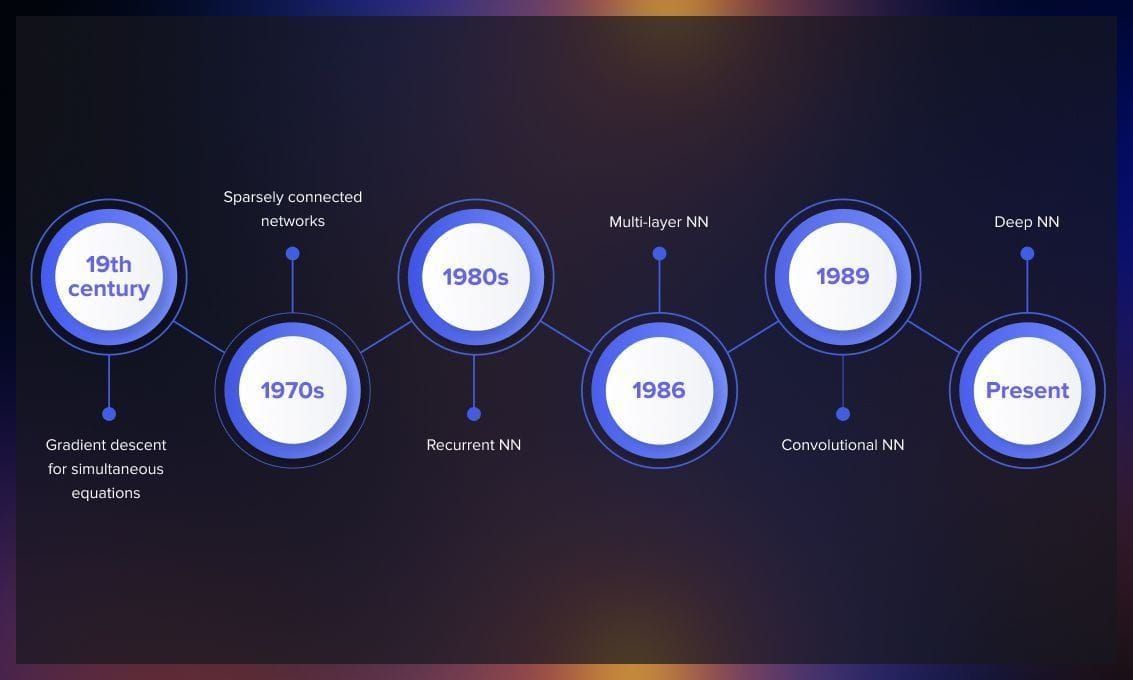
In the 19th century, Baron Augustin-Louis Cauchy, a French mathematician, developed a method called gradient descent to solve systems of simultaneous equations. His objective was to tackle complex astronomical calculations involving multiple variables. Cauchy’s idea was taking derivatives of a function and making small steps to minimize error.
Throughout the following century, gradient descent methods found applications across various disciplines, providing numerical solutions to challenging problems that would have been infeasible or computationally intractable to solve algebraically.
In 1970, Seppo Linnainmaa, a Finnish master’s student at the University of Helsinki, proposed an efficient algorithm for error backpropagation in sparsely connected networks. Although Linnainmaa did not specifically reference neural networks, his work laid the foundation for future developments.
In the 1980s, researchers independently developed backpropagation through time to enable the training of recurrent neural networks, further expanding the algorithm’s capabilities.
In 1986, David Rumelhart, an American psychologist, and his colleagues published a highly influential paper that applied Linnainmaa’s backpropagation algorithm to multi-layer neural networks. This marked a significant breakthrough; subsequent years witnessed further advancements built upon this algorithm. For instance, Yann LeCun’s 1989 paper demonstrated the application of backpropagation in convolutional neural networks for handwritten digit recognition.
In recent years, backpropagation plays a vital role in the efficient training of deep neural networks. While modifications have been made to parallelize the algorithm and leverage multiple GPUs, the original backpropagation algorithm developed by Linnainmaa and popularized by Rumelhart remains the fundamental backbone of contemporary deep learning-based artificial intelligence.
If you wish to have a more detailed, mathematically-based explanation of backpropagation, check out this article.
Conclusion
Backpropagation, as a core principle of deep learning, plays a significant role in many fields, where neural networks are involved. By facilitating the fine-tuning of weights within neural networks, it contributes to the generation of accurate predictions and classifications for nearly any industry. However, as with any technology, it’s essential to balance efficiency and complexity, understanding the algorithm’s limitations, such as the inability of gradient descent with backpropagation to recognize if it works with the global minimum of the error function or a local one, and difficulties crossing plateaus in the error function landscape.
To overcome these limitations, there have appeared new approaches and other optimizers, widely represented in the latest scientific papers. Check out some of the publications below.


.jpg)
.jpg)

