.png)
Imagine a scenario in which a model works perfectly well with the data it was trained on, but provides incorrect predictions when it meets new, unfamiliar data. On the other hand, in certain cases, it struggles to grasp the intricacies of the data and thus fails to provide an accurate prediction.
Striking a balance between accuracy and the ability to make predictions beyond the training data in an ML model is called the bias-variance tradeoff.
In this article, we will explore what bias and variance are, and how they affect the performance of machine learning models. We’ll also discuss techniques for balancing these two parameters and see how they can be applied in ML modeling.
What is bias?
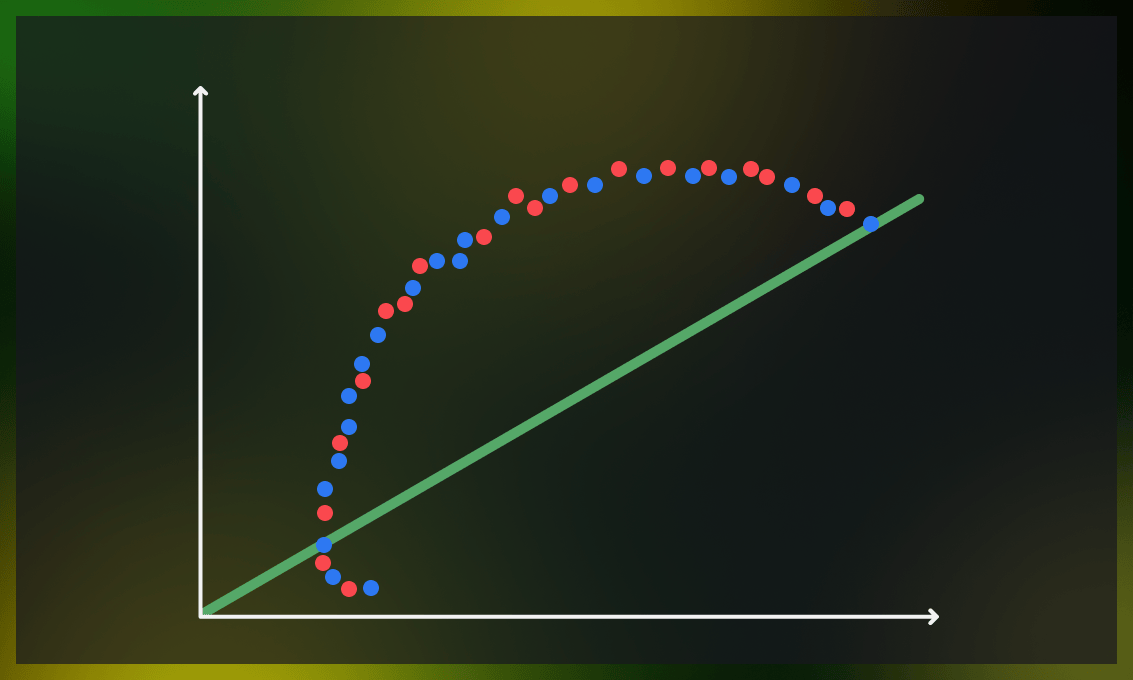
Bias in machine learning refers to the difference between a model’s predictions and the actual distribution of the value it tries to predict. Models with high bias oversimplify the data distribution rule/function, resulting in high errors in both the training outcomes and test data analysis results.
Bias is typically measured by evaluating the performance of a model on a training dataset. One common way to calculate bias is to use performance metrics such as mean squared error (MSE) or mean absolute error (MAE), which determine the difference between the predicted and real values of the training data.
Bias is a systematic error that occurs due to incorrect assumptions in the machine learning process, leading to the misrepresentation of data distribution.
The level of bias in a model is heavily influenced by the quality and quantity of training data involved. Using insufficient data will result in flawed predictions. At the same time, it can also result from the choice of an inappropriate model.
Watch this video for a more detailed explanation of how bias is measured:
High-bias model features
- Underfitting. High-bias models often underfit the data, meaning they oversimplify the solution based on generalization. As a result, the proposed distribution does not correspond to the actual distribution.
- Low training accuracy. The lack of proper processing of training data results in high training loss and low training accuracy.
- Oversimplification. The oversimplified nature of high-bias models limits their ability to identify complex features in the training data, making them inefficient for solving complicated problems.
Why is bias a problem?
Bias is problematic because it indicates that your model does not accurately represent the data it is trying to predict. However, in some situations, it may be acceptable to limit your model to a specific area, such as a specialized medical model for women under 30, or to add additional human control, such as calling an operator when the model is uncertain. The primary challenge is that you may be unable to identify all of these instances during the training and testing phase with complete certainty, which may result in unforeseen difficulties. Therefore, you should be prepared to address such issues as they arise.
How to reduce high bias?
There are several ways to overcome high bias:
- Incorporating additional features from data to improve the model’s accuracy.
- Increasing the number of training iterations to allow the model to learn more complex data.
- Avoiding high-bias algorithms such as linear regression, logistic regression, discriminant analysis, etc. and instead using nonlinear algorithms such as k-nearest neighbors, SVM, decision trees, etc.
- Decreasing regularization at various levels to help the model learn the training set more effectively and prevent underfitting.
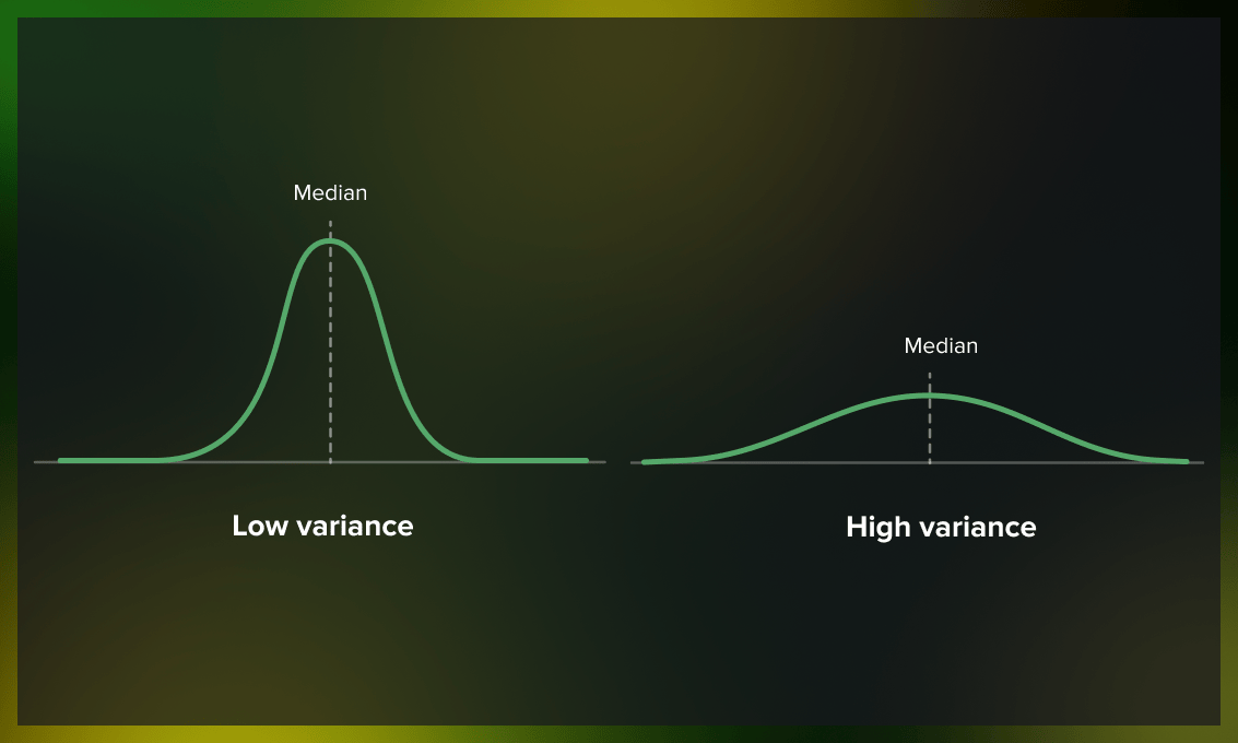
What is variance?
Variance stands in contrast to bias; it measures how much a distribution on several sets of data values differs from each other. The most common approach to measuring variance is by performing cross-validation experiments and looking at how the model performs on different random splits of your training data.
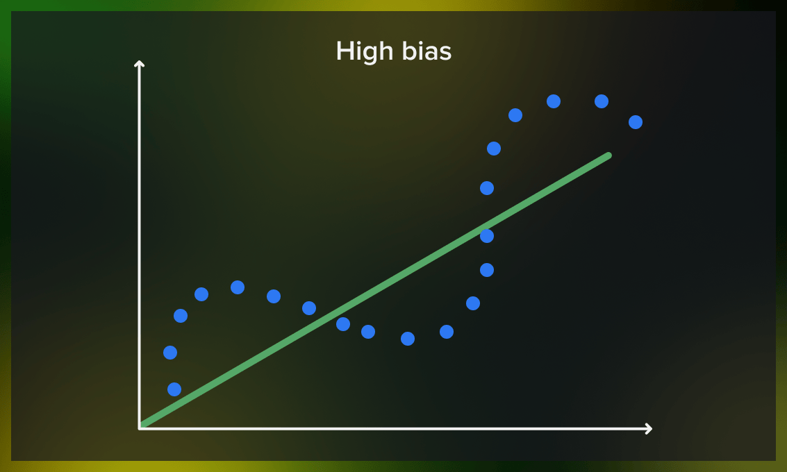
A model with a high level of variance depends heavily on the training data and, consequently, has a limited ability to generalize to new, unseen figures. This can result in excellent performance on training data but significantly higher error rates during model verification on the test data. Nonlinear machine learning algorithms often have high variance due to their high flexibility.
A complex model can learn complicated functions, which leads to higher variance. However, if the model becomes too complex for the dataset, high variance can result in overfitting. Low variance indicates a limited change in the target function in response to changes in the training data, while high variance means a significant difference.
High-variance model features
- Low testing accuracy. Despite high accuracy on training data, high variance models tend to perform poorly on test data.
- Overfitting. A high-variance model often leads to overfitting as it becomes too complex.
- Overcomplexity. As researchers, we expect that increasing the complexity of a model will result in improved performance on both training and testing data sets. However, when a model becomes too complex and a simpler model may provide the same level of accuracy, it’s better to choose the simpler one.
Model overcomplexity vs. model overfitting
Model overcomplexity and model overfitting are related, but they are not necessarily the same thing.
To put it simply, model overfitting occurs when a model is too complex for the distribution it is trying to predict. For instance, attempting to predict non-linear data with a linear model.
Model overcomplexity, on the other hand, happens when a model has too many parameters or a structure that is too complex to be effectively trained on the provided data. For instance, attempting to fit a neural network with 1.5 million parameters when only 100 objects are available. Such a model may fit the data well and have little bias, but it will likely have high variance as there is not enough data to capture the proper patterns with so many parameters.
Why is variance a problem?
Variance indicates that your model is not reliable. Suppose minor changes in the input data result in significant changes in the output. In that case, the model has not properly extracted the underlying patterns, and its decision making cannot be trusted. While having minor and predictable errors is acceptable, it’s a significant issue when the model performs well for some objects but completely fails for others. One possible approach to addressing this issue is to use a rule-based system in post-production, such as implementing a rule like “do not sell anything with a margin greater than 50%.”
How to reduce high variance?
The following methods can be used to overcome high variance:
- Reducing the number of features in the model.
- Replacing the current model with a simpler one.
- Increasing the training data diversity to balance out the complexity of the model and the data structure.
- Avoiding high-variance algorithms (support vector machines, decision trees, k-nearest neighbors, etc.) and opt for low-variance ones such as linear regression, logistic regression, and linear discriminant analysis.
- Performing hyperparameter tuning to avoid overfitting.
- Increasing regularization on inputs to decrease the complexity of the model and prevent overfitting.
- Using a new model architecture. (Like with the high bias, this should be considered a last resort if other methods are not effective.)
What bias-variance scenarios are possible?
Now let’s take a look at the different combinations of bias and variance in machine learning models and the results they provide.
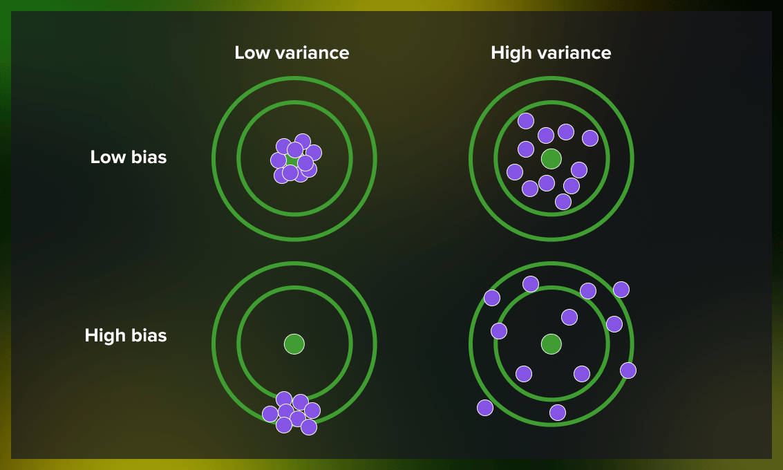
- Low bias, low variance: ideal model
A machine learning model with low bias and low variance is considered ideal but is not often the case in the machine learning practice, so we can speak of “reasonable bias” and “reasonable variance.”
- Low bias, high variance: results in overfitting
This combination results in inconsistent predictions that are accurate on average. It occurs when a model has too many parameters and fits too closely to the training data.
- High bias, low variance: results in underfitting
Predictions are consistent but inaccurate on average in this scenario. This happens when the model doesn’t learn well from the training data or has too few parameters, leading to underfitting issues.
- High bias, high variance: results in inaccurate predictions
With both high bias and high variance, the predictions are both inconsistent and inaccurate on average.
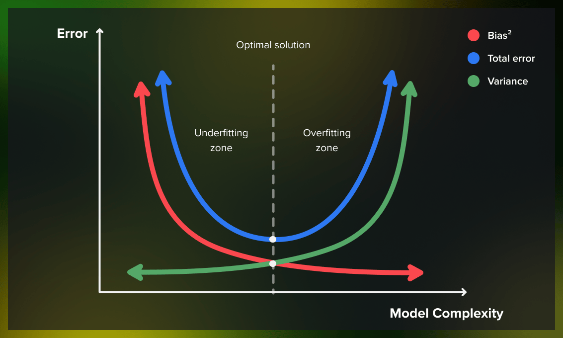
How to achieve a bias-variance tradeoff?
As we have learned, bias and variance are interdependent. In other words, lowering a model’s bias leads to an increase in its variance and vice versa. This relationship between bias and variance is known as the bias-variance tradeoff.
The balance between bias and variance can be adjusted in specific algorithms by modifying parameters, as seen in the following examples:
- For k-nearest neighbors, a low bias and high variance can be corrected by increasing the value of k, which increases the bias and decreases the variance.
- For support vector machines, a low bias and high variance can be altered by adjusting the C parameter, which increases the bias but decreases the variance.
Unfortunately, it’s impossible to determine the actual bias and variance error terms while we are trying to predict the target function. However, bias and variance serve as useful frameworks to understand the performance of machine learning algorithms in making predictions.
| Underfitting | Compromise | Overfitting | |
| Model Complexity | Low | Medium | High |
| Bias | High | Low | Low |
| Variance | Low | Low | High |
What is the difference between bias-variance decomposition and bias-variance tradeoff?
Bias-variance decomposition and bias-variance tradeoff are closely related concepts.
Bias-variance decomposition is a mathematical technique that divides the generalization error in a predictive model into two components: bias and variance.
In machine learning, as you try to minimize one component of the error (e.g., bias), the other component (e.g., variance) tends to increase, and vice versa. Finding the right balance of bias and variance is key to creating an effective and accurate model. This is called the bias-variance tradeoff.
Watch this video for a comprehensive explanation of the mathematical foundations behind bias- variance decomposition and the related underfitting or overfitting scenarios.
Using Python to achieve a good bias-variance tradeoff in the model
Setup
First, let’s import required libraries and set them up.
# general computations and data processing
import numpy as np
from sklearn.model_selection import train_test_split

# plotting
import matplotlib.pyplot as plt
import seaborn as sns
from matplotlib.animation import FuncAnimation, PillowWriter
# make matplotlib work inline and store images within the notebook
%matplotlib inline

# load default theme for Seaborn
sns.set()

# set random seed for reproducibility
np.random.seed(42)
Generating and plotting data
Next, let’s define the underlying function for the generated data, which we’ll later try to predict.
def f(X):
    y = -0.02 * X ** 4 + 0.1 * X ** 3 + 0.6 * X ** 2 - 1.2 * X + 2 * np.sin(X) + np.cos(X)
    string_representation = r"-0.02x^{4} + 0.1x^{3} + 0.6x^{2} - 1.2x + 2\sin(x) + \cos(x)"
    return y, string_representation
After that, we’ll define helper functions to work with this data.
generate_data will compute observed outcomes for provided input predictors , where is standard Gaussian noise.
def generate_data(input_predictors):
    white_noise = np.random.normal(size=input_predictors.shape)
    real_values, string_representation = f(input_predictors)
    # generate a title for the plot that will describe the way data is generated
    string_representation = fr"$y = {string_representation} + \varepsilon, \varepsilon \sim \mathcal{{N}}(0, 1)$"
    observed_outcomes = real_values + white_noise
    return real_values, observed_outcomes, string_representation
plot_generated_data will plot training data, test data and the underlying function.
def plot_generated_data(data, string_representation, test_data=None, true_data=None):
    figure, axes = plt.subplots(1, 1, figsize=(10, 8), dpi=200)
    # set general plot parameters
    axes.set_title(string_representation)
    axes.set_xlabel("Input predictors")
    axes.set_ylabel("Observed outcome")
    axes.grid(visible=True)
    # plot the data and the legend
    axes.scatter(data[0], data[1], marker=".", color="b", label="Train data")
    if test_data is not None:
        axes.scatter(test_data[0], test_data[1], marker=".", color="r", label="Test data")
    if true_data is not None:
        axes.plot(true_data[0], true_data[1], color="g", linewidth=1.5, label="Underlying function")
    axes.legend()
    # show the image and close the current figure
    plt.show()
    plt.close()
split_data will split generated observed outcomes into train and test datasets.
def split_data(X, y, f, test_split_size=0.2):
    X_train, X_test, y_train, y_test, f_train, f_test = train_test_split(X, y, f, test_size=test_split_size)
    return (X_train, y_train, f_train), (X_test, y_test, f_test)
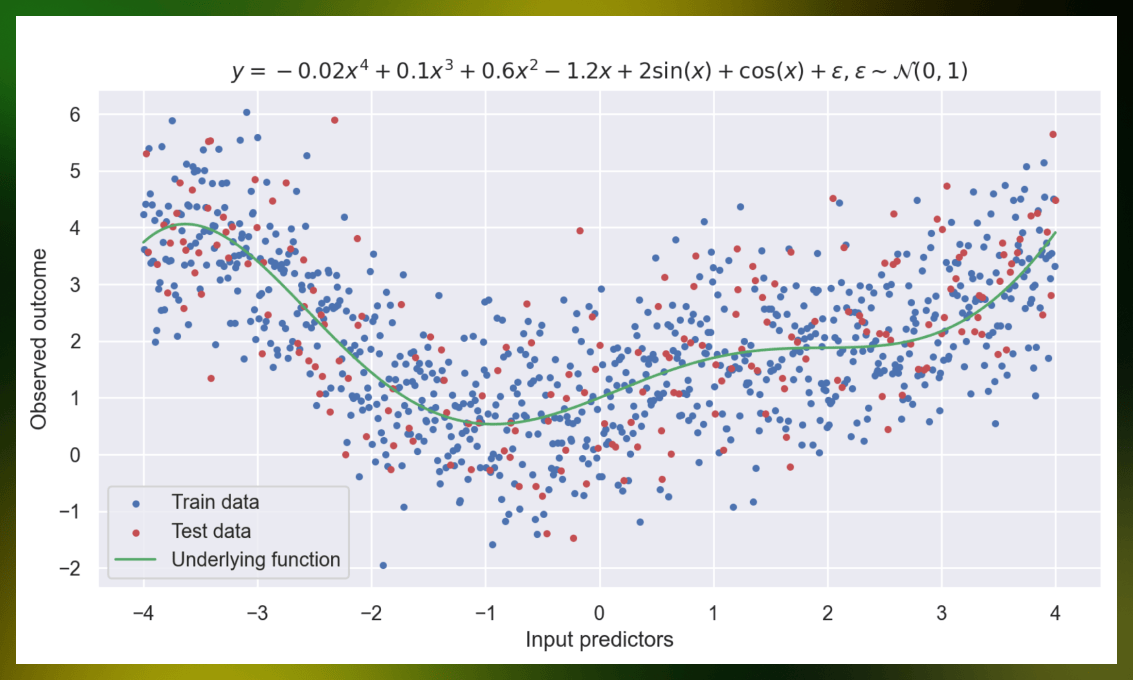
Next, we’ll use the functions to generate datapoints, split them into train and test sets, and plot them.
# generate 1000 points with noise that will become our dataset
input_predictors = np.linspace(-4, 4, 1000)
real_values, observed_outcomes, string_representation = generate_data(input_predictors)

# split them into train and test sets, the test set will contain 20% of all generated points
data_train, data_test = split_data(input_predictors, observed_outcomes, real_values)

# plot the data with the underlying function
plot_generated_data(data_train, string_representation, data_test, true_data=(input_predictors, real_values))
Plotting the bias-variance tradeoff
Let’s show the relation between bias and variance. We’ll fit polynomial regressions with different degrees of freedom using MSE as a loss function and compute bias and variance.
To compute them, we need to use a method called bootstrapping: we generate multiple subsets of the train dataset and train a model for each. After that, we can use predictions of those models on the test dataset to calculate bias and variance using the following formulas:
where is the learned model, is the input predictor, is the function that we want to predict. Note that the expectation is taken over both and .
max_polynomial_degree, num_bootstraps = 10, 1000

biases, variances, losses = [], [], []

for polynomial_degree in range(max_polynomial_degree):
    y_test_bootstrap_preds = []
    for _ in range(num_bootstraps):
        # get a random subset of train dataset
        bootstrap_idx = np.random.choice(len(data_train[0]), len(data_train[0]) // 5)
        # fit a polynomial regression model on said subset
        fit_coeff = np.polyfit(data_train[0][bootstrap_idx], data_train[1][bootstrap_idx], deg=polynomial_degree + 1)
        # collect predictions for test set generated by said model
        y_test_bootstrap_preds.append(np.polyval(fit_coeff, data_test[0]))
    # compute mean prediction over bootstraps
    mean_y_test_pred = np.mean(y_test_bootstrap_preds, axis=0)

    biases.append(((mean_y_test_pred - data_test[2]) ** 2).mean())
    variances.append(((y_test_bootstrap_preds - mean_y_test_pred) ** 2).mean())
    losses.append(((y_test_bootstrap_preds - data_test[1]) ** 2).mean(axis=1).mean())
For the sake of picture, we’ll plot squared bias.
best_polynomial_degree = np.argmin(losses)

fig, ax = plt.subplots(dpi=200)
ax.plot(np.arange(1, max_polynomial_degree + 1), biases, color="g", zorder=1)
ax.plot(np.arange(1, max_polynomial_degree + 1), losses, color="k", linestyle="--", label="Loss", zorder=1)
ax.set_ylabel("Bias", color="g")
ax.grid(visible=True, zorder=0)

ax2 = ax.twinx()
ax2.plot(np.arange(1, max_polynomial_degree + 1), variances, color="b", zorder=1)
ax2.set_ylabel("Variance", color="b")
ax2.grid(visible=False)

ax.scatter([best_polynomial_degree + 1], [losses[best_polynomial_degree]], color="r",  label=fr"Best model ($n = {best_polynomial_degree + 1}$)")
ax.set_xlabel("Polynomial Degree")
ax.set_title("Bias-variance tradeoff")
ax.legend(loc="upper center")
plt.show()
plt.close()
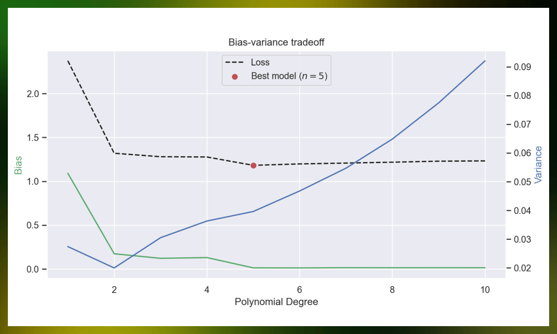
What does this plot say? When you increase model complexity, bias decreases, but variance increases. If you try to extend this plot to higher degrees, variance will explode.
Generally, you want to keep a certain balance between bias and variance. There are some cases when you don’t want that – for example, random forests. Each tree in a random forest is severely overfitted to minimize bias because the resulting prediction is a mean of predictions for each tree, so variance will decrease to reasonable levels.
As mentioned earlier, overly complicated models can get fairly low bias, but their variance will be enormous. Let’s visualize it by plotting best-fitted polynomials for different degrees.
To exacerbate the issue, we’ll enhance the noise on a few points in our training set and make them outliers. (It would be noticeable even without these shenanigans, but not to the same degree.)
train_subset = np.random.choice(len(data_train[0]), size=len(data_train[0]) // 80)
data_train[1][train_subset] += 49 * np.random.normal(size=len(data_train[0]) // 80)
Now, let’s animate how fitted polynomials change with increase in the degree of freedom.
# set up a figure to plot on
figure, ax = plt.subplots(1, 1, figsize=(10, 5), dpi=200)
fig.set_size_inches(5,4)

def animate_polynomial_fit(frame):
    # remove everything from current plot
    ax.clear()
    # fit a polynomial and get predictions for all points
    fit_coeff = np.polyfit(data_train[0], data_train[1], deg=frame + 1)
    y_pred = np.polyval(fit_coeff, input_predictors)
    # plot predicted polynomial, real function and test points
    ax.plot(input_predictors, y_pred, color="r", label=f"Predicted, degree = {frame + 1}")
    ax.plot(input_predictors, real_values, color="g", label="Real")
    ax.scatter(data_test[0], data_test[1], color="b", marker=".", label="Test points")
    # add description to the plot
    ax.set_title(r"Comparison between $f(x)$ and $\hat{f}(x)$")
    ax.set_xlabel("Input predictors")
    ax.set_ylabel("Observed outcome")
    ax.legend(loc="upper left")
    # set limits for the plot
    ax.set_xlim([-4, 4])
    ax.set_ylim([-1, 7])

# generate the animation
animation = FuncAnimation(figure, animate_polynomial_fit, frames=30, interval=500, repeat=False)
# save the animation as an animated GIF
animation.save("degree_change_animation.gif", dpi=300, writer=PillowWriter(fps=2))
At higher degrees, polynomials start “jumping around” the real value – they will heavily undershoot or overshoot in nearly every case. Why does this happen? Because the model begins to learn the noise as well, and we don’t want that.
Takeaway
In this post, you learned about bias, variance, and the trade-off between the two in the context of machine learning models. Let’s sum it up:
- Bias refers to the simplifying assumptions made by the model to make the target function more straightforward to approximate.
- Variance represents the degree to which the estimate of the target function varies when using different training data.
- The bias-variance tradeoff refers to a property of models where an increase in one component tends to result in a decrease in the other, and vice versa.
If you want to read more articles about ML, check out our machine learning section. And don’t forget to follow us on Twitter to stay updated about new articles we publish!


.jpg)
.jpg)